파이썬 데이터분석 - aarrr 분석 실습
- 고객의 정기예금 가입 여부 예측을 위한 은행 마케팅 분류 모델 구축
- 자전거 대여 수요 예측을 위한 머신러닝 모델 구축
- 파이썬 데이터분석 - A/B test 분석
- 파이썬 데이터분석 - 장바구니 분석(연관분석)2 - FP-Growth, 순차패턴마이닝
- 파이썬 데이터분석 - 장바구니 분석(연관분석) 실습
- 파이썬 데이터분석 - 장바구니 분석(연관분석)
- 파이썬 데이터분석 데이터시각화 실습
- 파이썬 데이터분석 데이터시각화2
- 파이썬 데이터분석 데이터시각화1
- 파이썬 데이터분석 클러스터와 차원축소 실습
- 파이썬 데이터분석 클러스터와 차원축소2
- 파이썬 데이터분석 클러스터와 차원축소
- 파이썬 데이터분석 라이브러리
1
2
3
4
import os
import pandas as pd
import numpy as np
import seaborn as sns
데이터 준비하기 + 전처리
- 실습내용 : 브라질의 이커머스 기업 Olist 데이터분석 (EDA + AARRR)
- 데이터출처 : 캐글
각 테이블 별로 간단한 EDA를 진행해보고 각 테이블이 어떤 의미와 특성을 가지고 있는지 파악하고, 테이블 간의 관계도 파악해보기
1. Customers (olist_customers_dataset.csv)
| 컬럼 이름 | 데이터 타입 | 설명 |
|---|---|---|
| customer_id | VARCHAR | 고객 고유 식별자 |
| customer_unique_id | VARCHAR | 고객의 고유 ID |
| customer_zip_code_prefix | INT | 고객의 우편번호 앞부분 |
| customer_city | VARCHAR | 고객의 도시 정보 |
| customer_state | VARCHAR | 고객의 주 정보 |
1
2
df = pd.read_csv('/content/drive/MyDrive/archive/olist_customers_dataset.csv')
df
| customer_id | customer_unique_id | customer_zip_code_prefix | customer_city | customer_state | |
|---|---|---|---|---|---|
| 0 | 06b8999e2fba1a1fbc88172c00ba8bc7 | 861eff4711a542e4b93843c6dd7febb0 | 14409 | franca | SP |
| 1 | 18955e83d337fd6b2def6b18a428ac77 | 290c77bc529b7ac935b93aa66c333dc3 | 9790 | sao bernardo do campo | SP |
| 2 | 4e7b3e00288586ebd08712fdd0374a03 | 060e732b5b29e8181a18229c7b0b2b5e | 1151 | sao paulo | SP |
| 3 | b2b6027bc5c5109e529d4dc6358b12c3 | 259dac757896d24d7702b9acbbff3f3c | 8775 | mogi das cruzes | SP |
| 4 | 4f2d8ab171c80ec8364f7c12e35b23ad | 345ecd01c38d18a9036ed96c73b8d066 | 13056 | campinas | SP |
| ... | ... | ... | ... | ... | ... |
| 99436 | 17ddf5dd5d51696bb3d7c6291687be6f | 1a29b476fee25c95fbafc67c5ac95cf8 | 3937 | sao paulo | SP |
| 99437 | e7b71a9017aa05c9a7fd292d714858e8 | d52a67c98be1cf6a5c84435bd38d095d | 6764 | taboao da serra | SP |
| 99438 | 5e28dfe12db7fb50a4b2f691faecea5e | e9f50caf99f032f0bf3c55141f019d99 | 60115 | fortaleza | CE |
| 99439 | 56b18e2166679b8a959d72dd06da27f9 | 73c2643a0a458b49f58cea58833b192e | 92120 | canoas | RS |
| 99440 | 274fa6071e5e17fe303b9748641082c8 | 84732c5050c01db9b23e19ba39899398 | 6703 | cotia | SP |
99441 rows × 5 columns
1
2
# 결측치 확인
df.isna().sum().sort_values(ascending=False)
| 0 | |
|---|---|
| customer_id | 0 |
| customer_unique_id | 0 |
| customer_zip_code_prefix | 0 |
| customer_city | 0 |
| customer_state | 0 |
1
2
# 중복값 확인
df.duplicated().sum()
1
0
1
2
# 중복값 확인
df['customer_id'].duplicated().sum()
1
0
1
df['customer_unique_id'].duplicated().sum()
1
3345
1
df[df['customer_unique_id'].duplicated(keep=False)].sort_values(by=['customer_unique_id'])
| customer_id | customer_unique_id | customer_zip_code_prefix | customer_city | customer_state | |
|---|---|---|---|---|---|
| 35608 | 24b0e2bd287e47d54d193e7bbb51103f | 00172711b30d52eea8b313a7f2cced02 | 45200 | jequie | BA |
| 19299 | 1afe8a9c67eec3516c09a8bdcc539090 | 00172711b30d52eea8b313a7f2cced02 | 45200 | jequie | BA |
| 20023 | 1b4a75b3478138e99902678254b260f4 | 004288347e5e88a27ded2bb23747066c | 26220 | nova iguacu | RJ |
| 22066 | f6efe5d5c7b85e12355f9d5c3db46da2 | 004288347e5e88a27ded2bb23747066c | 26220 | nova iguacu | RJ |
| 72451 | 49cf243e0d353cd418ca77868e24a670 | 004b45ec5c64187465168251cd1c9c2f | 57055 | maceio | AL |
| ... | ... | ... | ... | ... | ... |
| 75057 | 1ae563fdfa500d150be6578066d83998 | ff922bdd6bafcdf99cb90d7f39cea5b3 | 17340 | barra bonita | SP |
| 27992 | bec0bf00ac5bee64ce8ef5283051a70c | ff922bdd6bafcdf99cb90d7f39cea5b3 | 17340 | barra bonita | SP |
| 79859 | d064be88116eb8b958727aec4cf56a59 | ff922bdd6bafcdf99cb90d7f39cea5b3 | 17340 | barra bonita | SP |
| 64323 | 4b231c90751c27521f7ee27ed2dc3b8f | ffe254cc039740e17dd15a5305035928 | 37640 | extrema | MG |
| 12133 | 0088395699ea0fcd459bfbef084997db | ffe254cc039740e17dd15a5305035928 | 37640 | extrema | MG |
6342 rows × 5 columns
1
2
# 보유 고객중 2번이상 구매를 시도한 고객 비중은?
round(df['customer_unique_id'].duplicated().sum() / (df.shape[0] - df['customer_unique_id'].duplicated().sum()) * 100,2)
1
3.48
- 고객마다 고유 customer_unique_id가 있으며, 주문마다 고유의 customer_id가 생성된다
- customer_unique_id 중복값이 존재한다 → 2번이상 구매를 시도한 고객(재주문 혹은 주문취소포함 등) → 3,345명의 고객이 관찰됨 (약 3.5%)
- 대부분 1회성 고객임을 알 수 있다 → 재구매율을 높일지 회원수 확보를 높일지 전략을 세울필요가 있음
- customer_id컬럼과 orders데이터의 order_id컬럼이 1:1 매칭된다. 특정 고객이 주문하면 주문아이디와 매칭되는 커스텀아이디를 부여한다. 그렇기때문에 customer_id가 중복되는 경우는 존재하지 않는다
1
2
3
4
5
6
7
8
9
10
11
12
13
14
15
16
17
18
19
20
21
22
23
24
25
26
27
28
29
30
31
# 'customer_city'와 'customer_state' 상위 10 확인
city_counts = df['customer_city'].value_counts().head(10)
state_counts = df['customer_state'].value_counts().head(10)

# subplot 설정
fig, axs = plt.subplots(1, 2, figsize=(12, 5))

# 'customer_city' 그래프
axs[0].barh(city_counts.index[::-1], city_counts.values[::-1], color='skyblue')
axs[0].set_title('상위 10개 고객 도시')

# 빈도수 표시
for index, value in enumerate(city_counts.values[::-1]):
    axs[0].text(value, index, str(value))

axs[0].spines['top'].set_visible(False)
axs[0].spines['right'].set_visible(False)

# 'customer_state' 그래프
axs[1].barh(state_counts.index[::-1], state_counts.values[::-1], color='salmon')
axs[1].set_title('상위 10개 고객 주')

# 빈도수 표시
for index, value in enumerate(state_counts.values[::-1]):
    axs[1].text(value, index, str(value))

axs[1].spines['top'].set_visible(False)
axs[1].spines['right'].set_visible(False)

plt.tight_layout()
plt.show()
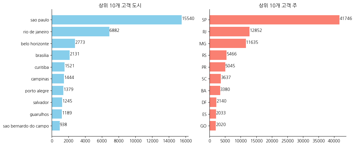
- olist고객 중 약 70%는 3개 주 (SP, RJ, MG)에 거주하고있고, 상파울로주(SP)는 전체 고객 중 43%가 거주하고있다
2. Orders (olist_orders_dataset.csv)
| 컬럼 이름 | 데이터 타입 | 설명 |
|---|---|---|
| order_id | VARCHAR | 주문 고유 식별자 |
| customer_id | VARCHAR | 고객 테이블과 연결되는 고객 식별자 |
| order_status | VARCHAR | 주문 상태 (배송 완료, 결제 완료 등) |
| order_purchase_timestamp | TIMESTAMP | 고객이 주문한 시각 |
| order_delivered_carrier_date | TIMESTAMP | 운송사가 배송을 시작한 시각 |
| order_delivered_customer_date | TIMESTAMP | 고객에게 최종 배송된 날짜 |
| order_estimated_delivery_date | TIMESTAMP | 예상 배송 날짜 |
1
2
df2 = pd.read_csv('/content/drive/MyDrive/archive/olist_orders_dataset.csv')
df2
| order_id | customer_id | order_status | order_purchase_timestamp | order_approved_at | order_delivered_carrier_date | order_delivered_customer_date | order_estimated_delivery_date | |
|---|---|---|---|---|---|---|---|---|
| 0 | e481f51cbdc54678b7cc49136f2d6af7 | 9ef432eb6251297304e76186b10a928d | delivered | 2017-10-02 10:56:33 | 2017-10-02 11:07:15 | 2017-10-04 19:55:00 | 2017-10-10 21:25:13 | 2017-10-18 00:00:00 |
| 1 | 53cdb2fc8bc7dce0b6741e2150273451 | b0830fb4747a6c6d20dea0b8c802d7ef | delivered | 2018-07-24 20:41:37 | 2018-07-26 03:24:27 | 2018-07-26 14:31:00 | 2018-08-07 15:27:45 | 2018-08-13 00:00:00 |
| 2 | 47770eb9100c2d0c44946d9cf07ec65d | 41ce2a54c0b03bf3443c3d931a367089 | delivered | 2018-08-08 08:38:49 | 2018-08-08 08:55:23 | 2018-08-08 13:50:00 | 2018-08-17 18:06:29 | 2018-09-04 00:00:00 |
| 3 | 949d5b44dbf5de918fe9c16f97b45f8a | f88197465ea7920adcdbec7375364d82 | delivered | 2017-11-18 19:28:06 | 2017-11-18 19:45:59 | 2017-11-22 13:39:59 | 2017-12-02 00:28:42 | 2017-12-15 00:00:00 |
| 4 | ad21c59c0840e6cb83a9ceb5573f8159 | 8ab97904e6daea8866dbdbc4fb7aad2c | delivered | 2018-02-13 21:18:39 | 2018-02-13 22:20:29 | 2018-02-14 19:46:34 | 2018-02-16 18:17:02 | 2018-02-26 00:00:00 |
| ... | ... | ... | ... | ... | ... | ... | ... | ... |
| 99436 | 9c5dedf39a927c1b2549525ed64a053c | 39bd1228ee8140590ac3aca26f2dfe00 | delivered | 2017-03-09 09:54:05 | 2017-03-09 09:54:05 | 2017-03-10 11:18:03 | 2017-03-17 15:08:01 | 2017-03-28 00:00:00 |
| 99437 | 63943bddc261676b46f01ca7ac2f7bd8 | 1fca14ff2861355f6e5f14306ff977a7 | delivered | 2018-02-06 12:58:58 | 2018-02-06 13:10:37 | 2018-02-07 23:22:42 | 2018-02-28 17:37:56 | 2018-03-02 00:00:00 |
| 99438 | 83c1379a015df1e13d02aae0204711ab | 1aa71eb042121263aafbe80c1b562c9c | delivered | 2017-08-27 14:46:43 | 2017-08-27 15:04:16 | 2017-08-28 20:52:26 | 2017-09-21 11:24:17 | 2017-09-27 00:00:00 |
| 99439 | 11c177c8e97725db2631073c19f07b62 | b331b74b18dc79bcdf6532d51e1637c1 | delivered | 2018-01-08 21:28:27 | 2018-01-08 21:36:21 | 2018-01-12 15:35:03 | 2018-01-25 23:32:54 | 2018-02-15 00:00:00 |
| 99440 | 66dea50a8b16d9b4dee7af250b4be1a5 | edb027a75a1449115f6b43211ae02a24 | delivered | 2018-03-08 20:57:30 | 2018-03-09 11:20:28 | 2018-03-09 22:11:59 | 2018-03-16 13:08:30 | 2018-04-03 00:00:00 |
99441 rows × 8 columns
1
2
# 결측치 확인
df2.isna().sum().sort_values(ascending=False)
| 0 | |
|---|---|
| order_delivered_customer_date | 2965 |
| order_delivered_carrier_date | 1783 |
| order_approved_at | 160 |
| order_id | 0 |
| customer_id | 0 |
| order_status | 0 |
| order_purchase_timestamp | 0 |
| order_estimated_delivery_date | 0 |
1
df2[df2['order_delivered_customer_date'].isna()]
| order_id | customer_id | order_status | order_purchase_timestamp | order_approved_at | order_delivered_carrier_date | order_delivered_customer_date | order_estimated_delivery_date | |
|---|---|---|---|---|---|---|---|---|
| 6 | 136cce7faa42fdb2cefd53fdc79a6098 | ed0271e0b7da060a393796590e7b737a | invoiced | 2017-04-11 12:22:08 | 2017-04-13 13:25:17 | NaN | NaN | 2017-05-09 00:00:00 |
| 44 | ee64d42b8cf066f35eac1cf57de1aa85 | caded193e8e47b8362864762a83db3c5 | shipped | 2018-06-04 16:44:48 | 2018-06-05 04:31:18 | 2018-06-05 14:32:00 | NaN | 2018-06-28 00:00:00 |
| 103 | 0760a852e4e9d89eb77bf631eaaf1c84 | d2a79636084590b7465af8ab374a8cf5 | invoiced | 2018-08-03 17:44:42 | 2018-08-07 06:15:14 | NaN | NaN | 2018-08-21 00:00:00 |
| 128 | 15bed8e2fec7fdbadb186b57c46c92f2 | f3f0e613e0bdb9c7cee75504f0f90679 | processing | 2017-09-03 14:22:03 | 2017-09-03 14:30:09 | NaN | NaN | 2017-10-03 00:00:00 |
| 154 | 6942b8da583c2f9957e990d028607019 | 52006a9383bf149a4fb24226b173106f | shipped | 2018-01-10 11:33:07 | 2018-01-11 02:32:30 | 2018-01-11 19:39:23 | NaN | 2018-02-07 00:00:00 |
| ... | ... | ... | ... | ... | ... | ... | ... | ... |
| 99283 | 3a3cddda5a7c27851bd96c3313412840 | 0b0d6095c5555fe083844281f6b093bb | canceled | 2018-08-31 16:13:44 | NaN | NaN | NaN | 2018-10-01 00:00:00 |
| 99313 | e9e64a17afa9653aacf2616d94c005b8 | b4cd0522e632e481f8eaf766a2646e86 | processing | 2018-01-05 23:07:24 | 2018-01-09 07:18:05 | NaN | NaN | 2018-02-06 00:00:00 |
| 99347 | a89abace0dcc01eeb267a9660b5ac126 | 2f0524a7b1b3845a1a57fcf3910c4333 | canceled | 2018-09-06 18:45:47 | NaN | NaN | NaN | 2018-09-27 00:00:00 |
| 99348 | a69ba794cc7deb415c3e15a0a3877e69 | 726f0894b5becdf952ea537d5266e543 | unavailable | 2017-08-23 16:28:04 | 2017-08-28 15:44:47 | NaN | NaN | 2017-09-15 00:00:00 |
| 99415 | 5fabc81b6322c8443648e1b21a6fef21 | 32c9df889d41b0ee8309a5efb6855dcb | unavailable | 2017-10-10 10:50:03 | 2017-10-14 18:35:57 | NaN | NaN | 2017-10-23 00:00:00 |
2965 rows × 8 columns
1
2
mask1 = df2[df2['order_delivered_customer_date'].isna()]
mask1['order_status'].value_counts()
| count | |
|---|---|
| order_status | |
| shipped | 1107 |
| canceled | 619 |
| unavailable | 609 |
| invoiced | 314 |
| processing | 301 |
| delivered | 8 |
| created | 5 |
| approved | 2 |
1
mask1[mask1['order_status'] == 'delivered']
| order_id | customer_id | order_status | order_purchase_timestamp | order_approved_at | order_delivered_carrier_date | order_delivered_customer_date | order_estimated_delivery_date | |
|---|---|---|---|---|---|---|---|---|
| 3002 | 2d1e2d5bf4dc7227b3bfebb81328c15f | ec05a6d8558c6455f0cbbd8a420ad34f | delivered | 2017-11-28 17:44:07 | 2017-11-28 17:56:40 | 2017-11-30 18:12:23 | NaN | 2017-12-18 00:00:00 |
| 20618 | f5dd62b788049ad9fc0526e3ad11a097 | 5e89028e024b381dc84a13a3570decb4 | delivered | 2018-06-20 06:58:43 | 2018-06-20 07:19:05 | 2018-06-25 08:05:00 | NaN | 2018-07-16 00:00:00 |
| 43834 | 2ebdfc4f15f23b91474edf87475f108e | 29f0540231702fda0cfdee0a310f11aa | delivered | 2018-07-01 17:05:11 | 2018-07-01 17:15:12 | 2018-07-03 13:57:00 | NaN | 2018-07-30 00:00:00 |
| 79263 | e69f75a717d64fc5ecdfae42b2e8e086 | cfda40ca8dd0a5d486a9635b611b398a | delivered | 2018-07-01 22:05:55 | 2018-07-01 22:15:14 | 2018-07-03 13:57:00 | NaN | 2018-07-30 00:00:00 |
| 82868 | 0d3268bad9b086af767785e3f0fc0133 | 4f1d63d35fb7c8999853b2699f5c7649 | delivered | 2018-07-01 21:14:02 | 2018-07-01 21:29:54 | 2018-07-03 09:28:00 | NaN | 2018-07-24 00:00:00 |
| 92643 | 2d858f451373b04fb5c984a1cc2defaf | e08caf668d499a6d643dafd7c5cc498a | delivered | 2017-05-25 23:22:43 | 2017-05-25 23:30:16 | NaN | NaN | 2017-06-23 00:00:00 |
| 97647 | ab7c89dc1bf4a1ead9d6ec1ec8968a84 | dd1b84a7286eb4524d52af4256c0ba24 | delivered | 2018-06-08 12:09:39 | 2018-06-08 12:36:39 | 2018-06-12 14:10:00 | NaN | 2018-06-26 00:00:00 |
| 98038 | 20edc82cf5400ce95e1afacc25798b31 | 28c37425f1127d887d7337f284080a0f | delivered | 2018-06-27 16:09:12 | 2018-06-27 16:29:30 | 2018-07-03 19:26:00 | NaN | 2018-07-19 00:00:00 |
1
2
mask2 = df2[~df2['order_delivered_customer_date'].isna()]
mask2['order_status'].value_counts()
| count | |
|---|---|
| order_status | |
| delivered | 96470 |
| canceled | 6 |
1
2
mask3 = df2[df2['order_delivered_carrier_date'].isna()]
mask3['order_status'].value_counts()
| count | |
|---|---|
| order_status | |
| unavailable | 609 |
| canceled | 550 |
| invoiced | 314 |
| processing | 301 |
| created | 5 |
| approved | 2 |
| delivered | 2 |
1
2
mask4 = df2[df2['order_approved_at'].isna()]
mask4['order_status'].value_counts()
| count | |
|---|---|
| order_status | |
| canceled | 141 |
| delivered | 14 |
| created | 5 |
- 일부 결측치가 관찰(배달이 완료됐는데 배송날짜가 안적혀있다던지 등)되었지만, 그 수가 100개 미만이고, 해당 결측치들에서 활용할수있는 유의미한 정보가(어떤것을 주문하고 판매됐고 가격, 카테고리 정보 등) 남아있다고 판단하기에 결측치를 제거하지않음
1
2
# 중복값 확인
df2.duplicated().sum()
1
0
1
df2['order_id'].duplicated().sum() + df2['customer_id'].duplicated().sum()
1
0
1
2
3
# customers 와 orders 데이터 customer_id 확인
merged_check_customer = pd.merge(df, df2, on='customer_id', how='outer', indicator=True)
merged_check_customer['_merge'].value_counts()
| count | |
|---|---|
| _merge | |
| both | 99441 |
| left_only | 0 |
| right_only | 0 |
- customers와 orders 데이터의 customer_id는 1:1로 정확히 매칭된다
- 다른데이터들과 order_id와 customer_id로 연결되고있다
1
df2['order_status'].value_counts()
| count | |
|---|---|
| order_status | |
| delivered | 96478 |
| shipped | 1107 |
| canceled | 625 |
| unavailable | 609 |
| invoiced | 314 |
| processing | 301 |
| created | 5 |
| approved | 2 |
1
round(df2[df2['order_status'] == 'canceled'].shape[0] / df2.shape[0] * 100, 2)
1
0.63
1
round(((df2[df2['order_status'] == 'canceled'].shape[0]) + (df2[df2['order_status'] == 'unavailable'].shape[0])) / df2.shape[0] * 100, 2)
1
1.24
- 대부분의 주문이 배달이 완료된 상황이고, 취소율은 0.6%(unavailable 포함시 1.2%)로 낮은수준으로 관찰됨
1
2
3
4
5
6
7
8
9
10
11
12
13
14
15
16
17
18
19
20
21
22
23
24
# 'order_purchase_timestamp' 컬럼을 datetime 형식으로 변환
df2['order_purchase_timestamp'] = pd.to_datetime(df2['order_purchase_timestamp'])

# 연도와 월별로 그룹화하여 주문 수 계산
monthly_orders = df2.groupby(df2['order_purchase_timestamp'].dt.to_period('M')).size()

# 시각화
plt.figure(figsize=(10, 6))
bars = plt.bar(monthly_orders.index.astype(str), monthly_orders.values, color='skyblue')

# 주문 수 표시
for bar in bars:
    yval = bar.get_height()
    plt.text(bar.get_x() + bar.get_width()/2, yval, str(yval), ha='center', va='bottom')

plt.title('월별 주문 수')
plt.xlabel('연도-월')
plt.ylabel('주문 수')
plt.xticks(rotation=45)
plt.grid(axis='y')

# 레이아웃 조정 및 그래프 표시
plt.tight_layout()
plt.show()
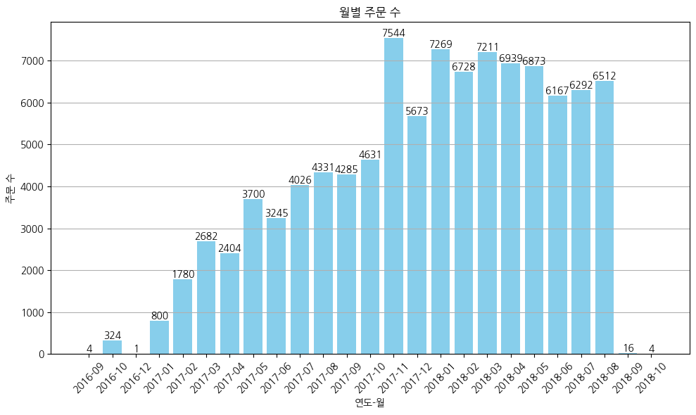
- 월별 주문수는 상승곡선을 보이고 있음
1
2
3
# 파생변수 배송기간 생성 (고객 배송일 - 고객 주문일 )
df2['order_delivered_customer_date'] = pd.to_datetime(df2['order_delivered_customer_date'])
df2['delivery_time'] = (df2['order_delivered_customer_date'] - df2['order_purchase_timestamp']).dt.days
1
2
3
4
5
6
7
8
9
10
11
12
13
14
15
plt.figure(figsize=(12, 6))
n, bins, patches = plt.hist(df2['delivery_time'], bins=range(0, int(df2['delivery_time'].max()) + 5, 5), color='skyblue', edgecolor='black')

for count, x in zip(n, bins):
    plt.text(x + 2.5, count, str(int(count)), ha='center', va='bottom')

plt.title('배송 기간 분포 (5일 단위)')
plt.xlabel('배송 기간 (일)')
plt.ylabel('주문 수')
plt.xticks(range(0, int(df2['delivery_time'].max()) + 5, 5))
plt.grid(axis='y')

# 레이아웃 조정 및 그래프 표시
plt.tight_layout()
plt.show()
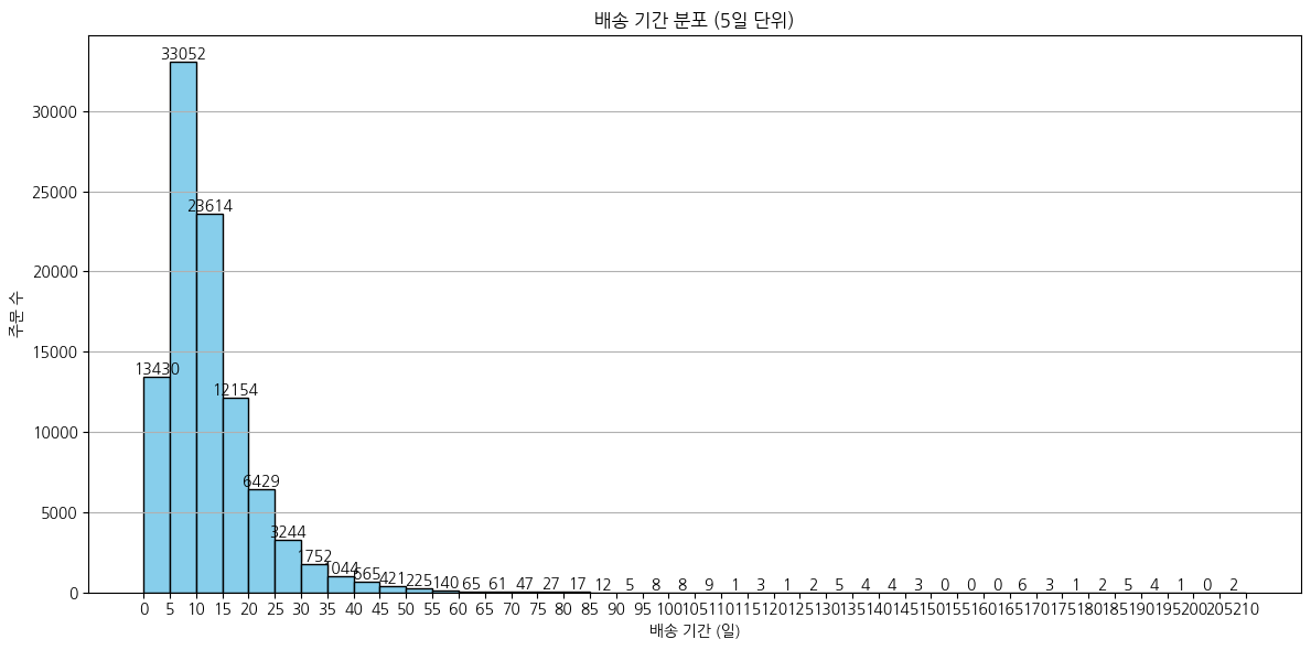
- 대부분 1달 이내 배달이 완료되고 5일~10일 분포가 가장 많음. 1달 뒤에 배송되는것도 일부 존재하고 배송에 2달 걸리는 배달도 다수있음
1
2
merged_df_delivery = pd.merge(df, df2[['customer_id', 'delivery_time']], on='customer_id', how='left')
merged_df_delivery
| customer_id | customer_unique_id | customer_zip_code_prefix | customer_city | customer_state | delivery_time | |
|---|---|---|---|---|---|---|
| 0 | 06b8999e2fba1a1fbc88172c00ba8bc7 | 861eff4711a542e4b93843c6dd7febb0 | 14409 | franca | SP | 8.0 |
| 1 | 18955e83d337fd6b2def6b18a428ac77 | 290c77bc529b7ac935b93aa66c333dc3 | 9790 | sao bernardo do campo | SP | 16.0 |
| 2 | 4e7b3e00288586ebd08712fdd0374a03 | 060e732b5b29e8181a18229c7b0b2b5e | 1151 | sao paulo | SP | 26.0 |
| 3 | b2b6027bc5c5109e529d4dc6358b12c3 | 259dac757896d24d7702b9acbbff3f3c | 8775 | mogi das cruzes | SP | 14.0 |
| 4 | 4f2d8ab171c80ec8364f7c12e35b23ad | 345ecd01c38d18a9036ed96c73b8d066 | 13056 | campinas | SP | 11.0 |
| ... | ... | ... | ... | ... | ... | ... |
| 99436 | 17ddf5dd5d51696bb3d7c6291687be6f | 1a29b476fee25c95fbafc67c5ac95cf8 | 3937 | sao paulo | SP | 6.0 |
| 99437 | e7b71a9017aa05c9a7fd292d714858e8 | d52a67c98be1cf6a5c84435bd38d095d | 6764 | taboao da serra | SP | 7.0 |
| 99438 | 5e28dfe12db7fb50a4b2f691faecea5e | e9f50caf99f032f0bf3c55141f019d99 | 60115 | fortaleza | CE | 30.0 |
| 99439 | 56b18e2166679b8a959d72dd06da27f9 | 73c2643a0a458b49f58cea58833b192e | 92120 | canoas | RS | 12.0 |
| 99440 | 274fa6071e5e17fe303b9748641082c8 | 84732c5050c01db9b23e19ba39899398 | 6703 | cotia | SP | 7.0 |
99441 rows × 6 columns
1
2
3
4
5
6
7
8
9
10
11
12
13
14
15
16
17
18
19
20
21
22
23
24
25
top_states = ['SP', 'RJ', 'MG']
fig, axs = plt.subplots(len(top_states), 1, figsize=(10, 15))

for i, state in enumerate(top_states):
    state_data = merged_df_delivery[merged_df_delivery['customer_state'] == state]

    # max 값을 int로 변환하여 range에 사용
    max_delivery_time = int(state_data['delivery_time'].max())

    axs[i].hist(state_data['delivery_time'],
                 bins=range(0, max_delivery_time + 10, 10),
                 color='skyblue', edgecolor='black', alpha=0.7)

    axs[i].set_title(f'{state} - 배송 기간 분포 (10일 단위)')
    axs[i].set_xlabel('배송 기간 (일)')
    axs[i].set_ylabel('주문 수')
    axs[i].grid(axis='y')

    # 각 막대 위에 카운트 표시
    counts, bins = np.histogram(state_data['delivery_time'], bins=range(0, max_delivery_time + 10, 10))
    for j in range(len(counts)):
        axs[i].text(bins[j] + 5, counts[j], str(counts[j]), ha='center', va='bottom')

plt.tight_layout()
plt.show()
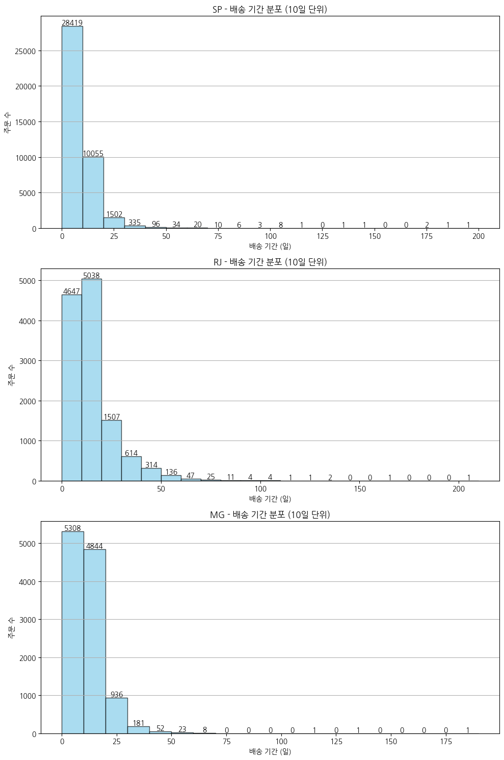
- 상위 3개 주 (전체 고객 중 70%) 배송기간은 RJ가 장기배송이 일부 있지만 대부분 20일 이내 배송되고 있음
3. Order Items (olist_order_items_dataset.csv)
| 컬럼 이름 | 데이터 타입 | 설명 |
|---|---|---|
| order_id | VARCHAR | 주문 고유 식별자 |
| order_item_id | INT | 주문 내에서의 각 상품의 식별자 |
| product_id | VARCHAR | 상품 고유 식별자 |
| seller_id | VARCHAR | 판매자 고유 식별자 |
| shipping_limit_date | TIMESTAMP | 판매자가 상품을 발송해야 하는 마감일 |
| price | FLOAT | 주문된 상품의 가격 |
| freight_value | FLOAT | 상품의 배송비 |
1
2
df3 = pd.read_csv('/content/drive/MyDrive/archive/olist_order_items_dataset.csv')
df3
| order_id | order_item_id | product_id | seller_id | shipping_limit_date | price | freight_value | |
|---|---|---|---|---|---|---|---|
| 0 | 00010242fe8c5a6d1ba2dd792cb16214 | 1 | 4244733e06e7ecb4970a6e2683c13e61 | 48436dade18ac8b2bce089ec2a041202 | 2017-09-19 09:45:35 | 58.90 | 13.29 |
| 1 | 00018f77f2f0320c557190d7a144bdd3 | 1 | e5f2d52b802189ee658865ca93d83a8f | dd7ddc04e1b6c2c614352b383efe2d36 | 2017-05-03 11:05:13 | 239.90 | 19.93 |
| 2 | 000229ec398224ef6ca0657da4fc703e | 1 | c777355d18b72b67abbeef9df44fd0fd | 5b51032eddd242adc84c38acab88f23d | 2018-01-18 14:48:30 | 199.00 | 17.87 |
| 3 | 00024acbcdf0a6daa1e931b038114c75 | 1 | 7634da152a4610f1595efa32f14722fc | 9d7a1d34a5052409006425275ba1c2b4 | 2018-08-15 10:10:18 | 12.99 | 12.79 |
| 4 | 00042b26cf59d7ce69dfabb4e55b4fd9 | 1 | ac6c3623068f30de03045865e4e10089 | df560393f3a51e74553ab94004ba5c87 | 2017-02-13 13:57:51 | 199.90 | 18.14 |
| ... | ... | ... | ... | ... | ... | ... | ... |
| 112645 | fffc94f6ce00a00581880bf54a75a037 | 1 | 4aa6014eceb682077f9dc4bffebc05b0 | b8bc237ba3788b23da09c0f1f3a3288c | 2018-05-02 04:11:01 | 299.99 | 43.41 |
| 112646 | fffcd46ef2263f404302a634eb57f7eb | 1 | 32e07fd915822b0765e448c4dd74c828 | f3c38ab652836d21de61fb8314b69182 | 2018-07-20 04:31:48 | 350.00 | 36.53 |
| 112647 | fffce4705a9662cd70adb13d4a31832d | 1 | 72a30483855e2eafc67aee5dc2560482 | c3cfdc648177fdbbbb35635a37472c53 | 2017-10-30 17:14:25 | 99.90 | 16.95 |
| 112648 | fffe18544ffabc95dfada21779c9644f | 1 | 9c422a519119dcad7575db5af1ba540e | 2b3e4a2a3ea8e01938cabda2a3e5cc79 | 2017-08-21 00:04:32 | 55.99 | 8.72 |
| 112649 | fffe41c64501cc87c801fd61db3f6244 | 1 | 350688d9dc1e75ff97be326363655e01 | f7ccf836d21b2fb1de37564105216cc1 | 2018-06-12 17:10:13 | 43.00 | 12.79 |
112650 rows × 7 columns
1
2
# 결측치 확인
df3.isna().sum().sort_values(ascending=False)
| 0 | |
|---|---|
| order_id | 0 |
| order_item_id | 0 |
| product_id | 0 |
| seller_id | 0 |
| shipping_limit_date | 0 |
| price | 0 |
| freight_value | 0 |
1
2
# 중복값 확인
df3.duplicated().sum()
1
0
1
df3['order_id'].duplicated().sum()
1
13984
1
df3[df3['order_id'].duplicated()].sort_values(by=['product_id', 'order_item_id'])
| order_id | order_item_id | product_id | seller_id | shipping_limit_date | price | freight_value | |
|---|---|---|---|---|---|---|---|
| 82591 | bb9552306cf6879fde49f4ba3bd94299 | 2 | 0011c512eb256aa0dbbb544d8dffcf6e | b4ffb71f0cb1b1c3d63fad021ecf93e1 | 2017-12-22 20:38:29 | 52.00 | 15.80 |
| 86374 | c432657bb18ddf7f48b7227db09048d4 | 2 | 001795ec6f1b187d37335e1c4704762e | 8b321bb669392f5163d04c59e235e066 | 2017-12-18 00:39:25 | 38.90 | 16.11 |
| 97530 | dd436680fbd2d38edb26277f5b8379dc | 2 | 001795ec6f1b187d37335e1c4704762e | 8b321bb669392f5163d04c59e235e066 | 2017-12-29 15:30:50 | 38.90 | 9.34 |
| 49689 | 70ed857e24fd6bf1e25a9bc791a2f6b9 | 2 | 001b72dfd63e9833e8c02742adf472e3 | 8a32e327fe2c1b3511609d81aaf9f042 | 2017-09-06 12:35:16 | 34.99 | 9.90 |
| 85437 | c214276ccd69c3953f880b487209f47e | 2 | 001b72dfd63e9833e8c02742adf472e3 | 8a32e327fe2c1b3511609d81aaf9f042 | 2017-07-13 15:43:15 | 34.99 | 7.78 |
| ... | ... | ... | ... | ... | ... | ... | ... |
| 56508 | 808b7fff91e537a5df90717957ee5bb1 | 2 | ffef256879dbadcab7e77950f4f4a195 | 113e3a788b935f48aad63e1c41dac1bd | 2018-06-15 19:54:42 | 31.78 | 18.23 |
| 83782 | be48bdef069ed1eb0d320bfe65d26351 | 2 | fff0a542c3c62682f23305214eaeaa24 | 08d2d642cf72b622b14dde1d2f5eb2f5 | 2017-12-07 19:53:44 | 7.50 | 12.69 |
| 106253 | f179e0782e0180bc2ec9ce167d4cf245 | 2 | fff0a542c3c62682f23305214eaeaa24 | 08d2d642cf72b622b14dde1d2f5eb2f5 | 2017-12-12 02:35:39 | 7.50 | 16.11 |
| 106254 | f179e0782e0180bc2ec9ce167d4cf245 | 3 | fff0a542c3c62682f23305214eaeaa24 | 08d2d642cf72b622b14dde1d2f5eb2f5 | 2017-12-12 02:35:39 | 7.50 | 16.11 |
| 106255 | f179e0782e0180bc2ec9ce167d4cf245 | 4 | fff0a542c3c62682f23305214eaeaa24 | 08d2d642cf72b622b14dde1d2f5eb2f5 | 2017-12-12 02:35:39 | 7.50 | 16.11 |
13984 rows × 7 columns
1
df3.sort_values(by=['order_item_id'])
| order_id | order_item_id | product_id | seller_id | shipping_limit_date | price | freight_value | |
|---|---|---|---|---|---|---|---|
| 0 | 00010242fe8c5a6d1ba2dd792cb16214 | 1 | 4244733e06e7ecb4970a6e2683c13e61 | 48436dade18ac8b2bce089ec2a041202 | 2017-09-19 09:45:35 | 58.90 | 13.29 |
| 72706 | a5c7406fd66b64f69acd95538f35b97e | 1 | 06edb72f1e0c64b14c5b79353f7abea3 | 391fc6631aebcf3004804e51b40bcf1e | 2017-08-28 21:25:19 | 45.95 | 15.10 |
| 72705 | a5c681209e1bcb90066e530c285ce2c5 | 1 | eec68ed7d496bb2ee6aa0a69bb78acd2 | 5f5b43b2bffa8656e4bc6efeb13cc649 | 2017-12-21 20:51:36 | 89.00 | 9.44 |
| 72704 | a5c654c2a0126153f98af71a65a159de | 1 | b37a8cda46313ac91d79f16601ca5253 | 955fee9216a65b617aa5c0531780ce60 | 2018-06-12 12:10:35 | 95.00 | 20.72 |
| 72703 | a5c523f7f14f85ee88f26643f9a99e66 | 1 | 4b96786612ebe7463132fce2c4dca136 | d94a40fd42351c259927028d163af842 | 2018-06-14 08:31:15 | 129.00 | 26.05 |
| ... | ... | ... | ... | ... | ... | ... | ... |
| 11950 | 1b15974a0141d54e36626dca3fdc731a | 19 | ee3d532c8a438679776d222e997606b3 | 8e6d7754bc7e0f22c96d255ebda59eba | 2018-03-01 02:50:48 | 100.00 | 10.12 |
| 11951 | 1b15974a0141d54e36626dca3fdc731a | 20 | ee3d532c8a438679776d222e997606b3 | 8e6d7754bc7e0f22c96d255ebda59eba | 2018-03-01 02:50:48 | 100.00 | 10.12 |
| 75122 | ab14fdcfbe524636d65ee38360e22ce8 | 20 | 9571759451b1d780ee7c15012ea109d4 | ce27a3cc3c8cc1ea79d11e561e9bebb6 | 2017-08-30 14:30:23 | 98.70 | 14.44 |
| 57316 | 8272b63d03f5f79c56e9e4120aec44ef | 20 | 270516a3f41dc035aa87d220228f844c | 2709af9587499e95e803a6498a5a56e9 | 2017-07-21 18:25:23 | 1.20 | 7.89 |
| 57317 | 8272b63d03f5f79c56e9e4120aec44ef | 21 | 79ce45dbc2ea29b22b5a261bbb7b7ee7 | 2709af9587499e95e803a6498a5a56e9 | 2017-07-21 18:25:23 | 7.80 | 6.57 |
112650 rows × 7 columns
1
df3[df3['product_id'] == 'fff0a542c3c62682f23305214eaeaa24']
| order_id | order_item_id | product_id | seller_id | shipping_limit_date | price | freight_value | |
|---|---|---|---|---|---|---|---|
| 31855 | 4838d1c1cbef87593a3921429e633ccc | 1 | fff0a542c3c62682f23305214eaeaa24 | 08d2d642cf72b622b14dde1d2f5eb2f5 | 2017-11-17 20:50:31 | 7.3 | 15.10 |
| 47963 | 6d03ab0713a35b9475f6c5ed0d989976 | 1 | fff0a542c3c62682f23305214eaeaa24 | 08d2d642cf72b622b14dde1d2f5eb2f5 | 2017-12-07 14:11:22 | 7.5 | 16.11 |
| 83781 | be48bdef069ed1eb0d320bfe65d26351 | 1 | fff0a542c3c62682f23305214eaeaa24 | 08d2d642cf72b622b14dde1d2f5eb2f5 | 2017-12-07 19:53:44 | 7.5 | 12.69 |
| 83782 | be48bdef069ed1eb0d320bfe65d26351 | 2 | fff0a542c3c62682f23305214eaeaa24 | 08d2d642cf72b622b14dde1d2f5eb2f5 | 2017-12-07 19:53:44 | 7.5 | 12.69 |
| 106252 | f179e0782e0180bc2ec9ce167d4cf245 | 1 | fff0a542c3c62682f23305214eaeaa24 | 08d2d642cf72b622b14dde1d2f5eb2f5 | 2017-12-12 02:35:39 | 7.5 | 16.11 |
| 106253 | f179e0782e0180bc2ec9ce167d4cf245 | 2 | fff0a542c3c62682f23305214eaeaa24 | 08d2d642cf72b622b14dde1d2f5eb2f5 | 2017-12-12 02:35:39 | 7.5 | 16.11 |
| 106254 | f179e0782e0180bc2ec9ce167d4cf245 | 3 | fff0a542c3c62682f23305214eaeaa24 | 08d2d642cf72b622b14dde1d2f5eb2f5 | 2017-12-12 02:35:39 | 7.5 | 16.11 |
| 106255 | f179e0782e0180bc2ec9ce167d4cf245 | 4 | fff0a542c3c62682f23305214eaeaa24 | 08d2d642cf72b622b14dde1d2f5eb2f5 | 2017-12-12 02:35:39 | 7.5 | 16.11 |
- 같은 주문번호/상품번호는 같은 상품을 n개 샀다는 의미이다 → 해당주문번호의 payment_value값과 (price + freight_value)*n이 동일함
- 또한, 같은 상품번호는 해당 상품을 현재 데이터기간동안(2016년~2018년) n개 판매했다는 의미이다. 예시에서 ‘fff0a542c3c62682f23305214eaeaa24’ 상품이 총 8번 판매되었다
1
df3['order_item_id'].value_counts()
| count | |
|---|---|
| order_item_id | |
| 1 | 98666 |
| 2 | 9803 |
| 3 | 2287 |
| 4 | 965 |
| 5 | 460 |
| 6 | 256 |
| 7 | 58 |
| 8 | 36 |
| 9 | 28 |
| 10 | 25 |
| 11 | 17 |
| 12 | 13 |
| 13 | 8 |
| 14 | 7 |
| 15 | 5 |
| 16 | 3 |
| 17 | 3 |
| 18 | 3 |
| 19 | 3 |
| 20 | 3 |
| 21 | 1 |
- order_item_id가 order 데이터의 order_id 수보다 775개 작다 (99441 > 98666)
1
2
3
4
5
6
7
8
not_in_df2 = df3[~df3['order_id'].isin(df2['order_id'])]
not_in_df3 = df2[~df2['order_id'].isin(df3['order_id'])]

print("df3에만 있는 order_id:")
print(not_in_df2['order_id'])

print("\ndf2에만 있는 order_id:")
print(not_in_df3['order_id'])
1
2
3
4
5
6
7
8
9
10
11
12
13
14
15
16
df3에만 있는 order_id:
Series([], Name: order_id, dtype: object)

df2에만 있는 order_id:
266      8e24261a7e58791d10cb1bf9da94df5c
586      c272bcd21c287498b4883c7512019702
687      37553832a3a89c9b2db59701c357ca67
737      d57e15fb07fd180f06ab3926b39edcd2
1130     00b1cb0320190ca0daa2c88b35206009
                       ...
99252    aaab15da689073f8f9aa978a390a69d1
99283    3a3cddda5a7c27851bd96c3313412840
99347    a89abace0dcc01eeb267a9660b5ac126
99348    a69ba794cc7deb415c3e15a0a3877e69
99415    5fabc81b6322c8443648e1b21a6fef21
Name: order_id, Length: 775, dtype: object
1
2
# order_items에 없는 주문들은 무엇일까
not_in_df3
| order_id | customer_id | order_status | order_purchase_timestamp | order_approved_at | order_delivered_carrier_date | order_delivered_customer_date | order_estimated_delivery_date | delivery_time | |
|---|---|---|---|---|---|---|---|---|---|
| 266 | 8e24261a7e58791d10cb1bf9da94df5c | 64a254d30eed42cd0e6c36dddb88adf0 | unavailable | 2017-11-16 15:09:28 | 2017-11-16 15:26:57 | NaN | NaT | 2017-12-05 00:00:00 | NaN |
| 586 | c272bcd21c287498b4883c7512019702 | 9582c5bbecc65eb568e2c1d839b5cba1 | unavailable | 2018-01-31 11:31:37 | 2018-01-31 14:23:50 | NaN | NaT | 2018-02-16 00:00:00 | NaN |
| 687 | 37553832a3a89c9b2db59701c357ca67 | 7607cd563696c27ede287e515812d528 | unavailable | 2017-08-14 17:38:02 | 2017-08-17 00:15:18 | NaN | NaT | 2017-09-05 00:00:00 | NaN |
| 737 | d57e15fb07fd180f06ab3926b39edcd2 | 470b93b3f1cde85550fc74cd3a476c78 | unavailable | 2018-01-08 19:39:03 | 2018-01-09 07:26:08 | NaN | NaT | 2018-02-06 00:00:00 | NaN |
| 1130 | 00b1cb0320190ca0daa2c88b35206009 | 3532ba38a3fd242259a514ac2b6ae6b6 | canceled | 2018-08-28 15:26:39 | NaN | NaN | NaT | 2018-09-12 00:00:00 | NaN |
| ... | ... | ... | ... | ... | ... | ... | ... | ... | ... |
| 99252 | aaab15da689073f8f9aa978a390a69d1 | df20748206e4b865b2f14a5eabbfcf34 | unavailable | 2018-01-16 14:27:59 | 2018-01-17 03:37:34 | NaN | NaT | 2018-02-06 00:00:00 | NaN |
| 99283 | 3a3cddda5a7c27851bd96c3313412840 | 0b0d6095c5555fe083844281f6b093bb | canceled | 2018-08-31 16:13:44 | NaN | NaN | NaT | 2018-10-01 00:00:00 | NaN |
| 99347 | a89abace0dcc01eeb267a9660b5ac126 | 2f0524a7b1b3845a1a57fcf3910c4333 | canceled | 2018-09-06 18:45:47 | NaN | NaN | NaT | 2018-09-27 00:00:00 | NaN |
| 99348 | a69ba794cc7deb415c3e15a0a3877e69 | 726f0894b5becdf952ea537d5266e543 | unavailable | 2017-08-23 16:28:04 | 2017-08-28 15:44:47 | NaN | NaT | 2017-09-15 00:00:00 | NaN |
| 99415 | 5fabc81b6322c8443648e1b21a6fef21 | 32c9df889d41b0ee8309a5efb6855dcb | unavailable | 2017-10-10 10:50:03 | 2017-10-14 18:35:57 | NaN | NaT | 2017-10-23 00:00:00 | NaN |
775 rows × 9 columns
1
2
3
4
print(not_in_df3['order_status'].value_counts())
print(not_in_df3['order_purchase_timestamp'].isna().sum())
print(not_in_df3['order_delivered_carrier_date'].unique())
print(not_in_df3['order_delivered_customer_date'].unique())
1
2
3
4
5
6
7
8
9
10
11
12
order_status
unavailable    603
canceled       164
created          5
invoiced         2
shipped          1
Name: count, dtype: int64
0
[nan '2016-11-07 16:37:37']
<DatetimeArray>
['NaT']
Length: 1, dtype: datetime64[ns]
1
not_in_df3[not_in_df3['order_status'] == 'shipped']
| order_id | customer_id | order_status | order_purchase_timestamp | order_approved_at | order_delivered_carrier_date | order_delivered_customer_date | order_estimated_delivery_date | delivery_time | |
|---|---|---|---|---|---|---|---|---|---|
| 23254 | a68ce1686d536ca72bd2dadc4b8671e5 | d7bed5fac093a4136216072abaf599d5 | shipped | 2016-10-05 01:47:40 | 2016-10-07 03:11:22 | 2016-11-07 16:37:37 | NaT | 2016-12-01 00:00:00 | NaN |
- 상품 취소나 시스템 오류 등으로 주문번호는 남아있지만 최종적으로 고객에게 배송되지않고 상품관련정보도 전부삭제된 데이터이다. 결측치로 제거할수도있지만, 사용자가 구매시도한 데이터에는 결측치가 없었다. 따라서 사용자가 구매를 시도한후 변경된 데이터들이다. 따라서 해당 데이터를 제거하지 않기로 결정함
1
df3['shipping_limit_date'].isna().sum()
1
0
1
df3['shipping_limit_date'].describe()
| shipping_limit_date | |
|---|---|
| count | 112650 |
| unique | 93318 |
| top | 2017-07-21 18:25:23 |
| freq | 21 |
1
(df3['freight_value'] > df3['price']).sum()
1
4124
- 상품보다 배송비가 더 비싼 건이 전체 거래 대비 약 4% 발생한것으로 관찰됨
1
2
3
4
5
6
7
8
9
10
11
12
13
14
15
16
17
18
19
20
21
22
23
24
25
26
27
28
29
30
31
32
33
34
35
36
37
38
39
40
41
42
43
44
45
46
47
48
# 연도와 월별로 그룹화하여 주문 수 계산
monthly_orders = df2.groupby(df2['order_purchase_timestamp'].dt.to_period('M')).size()

# 1. 'shipping_limit_date'를 datetime 형식으로 변환
df3['shipping_limit_date'] = pd.to_datetime(df3['shipping_limit_date'])

# 2. 월별 매출액 집계
monthly_sales = df3.resample('M', on='shipping_limit_date')['price'].sum()

# 3. 2018년 8월까지의 데이터만 필터링
monthly_sales = monthly_sales[monthly_sales.index <= '2018-08-31']

# 4. subplot 생성
fig, (ax1, ax2) = plt.subplots(2, 1, figsize=(10, 12))

# 첫 번째 차트: 월별 주문 수
bars = ax1.bar(monthly_orders.index.astype(str), monthly_orders.values, color='skyblue')

# 주문 수 표시
for bar in bars:
    yval = bar.get_height()
    ax1.text(bar.get_x() + bar.get_width()/2, yval, str(yval), ha='center', va='bottom')

ax1.set_title('월별 주문 수')
ax1.set_xlabel('연도-월')
ax1.set_ylabel('주문 수')
ax1.set_xticks(range(len(monthly_orders.index)))  # x축 위치 설정
ax1.set_xticklabels(monthly_orders.index.astype(str), rotation=45)  # 레이블과 회전 설정
ax1.grid(axis='y')

# 두 번째 차트: 월별 매출액 추이
ax2.plot(monthly_sales.index, monthly_sales.values, marker='o')

# 매출액 숫자 표기
for x, y in zip(monthly_sales.index, monthly_sales.values):
    ax2.text(x, y, f'{y:,.0f}', fontsize=9, ha='center', va='bottom')

# x축을 3개월 단위로 설정
ax2.set_xticks(monthly_sales.index[::3])
ax2.set_title('월별 매출액 추이')
ax2.set_xlabel('월')
ax2.set_ylabel('매출액')
ax2.set_xlim(pd.Timestamp('2016-09-01'), pd.Timestamp('2018-08-31'))  # x축 범위 설정
ax2.grid()

# 레이아웃 조정 및 그래프 표시
plt.tight_layout()
plt.show()

1
2
3
4
5
6
7
8
9
10
11
12
13
14
15
16
17
18
19
20
21
22
23
24
25
26
27
28
29
30
31
32
33
34
35
36
37
38
39
40
41
42
43
44
45
# 1. 상품별 판매 빈도수와 총 매출액 계산
product_sales = df3.groupby('product_id').agg(
    sales_count=('price', 'size'),  # 판매 빈도수
    total_revenue=('price', 'sum')  # 총 매출액
).reset_index()

# 2. 총 매출액 기준으로 정렬하고 상위 10개 선택
top_products = product_sales.sort_values(by='total_revenue', ascending=False).head(10)

# 3. 상품 순서를 총 매출액 기준으로 역순으로 설정
top_products = top_products.sort_values(by='total_revenue', ascending=True)

# 4. subplot 생성
fig, (ax1, ax2) = plt.subplots(1, 2, figsize=(12, 6))

# 5. 왼쪽 차트: 총 매출액
bars1 = ax1.barh(top_products['product_id'], top_products['total_revenue'], color='skyblue')
ax1.set_title('상품별 총 매출액 (상위 10개 상품)')
ax1.set_xlabel('총 매출액')
ax1.grid(axis='x')
ax1.spines['top'].set_visible(False)
ax1.spines['right'].set_visible(False)

# 6. 숫자 표기
for bar in bars1:
    ax1.text(bar.get_width(), bar.get_y() + bar.get_height()/2, f'{bar.get_width():,.0f}',
             va='center', ha='left', fontsize=9)

# 7. 오른쪽 차트: 판매 빈도수
bars2 = ax2.barh(top_products['product_id'], top_products['sales_count'], color='lightgreen')
ax2.set_title('상품별 판매 빈도수 (상위 10개 상품)')
ax2.set_xlabel('판매 빈도수')
ax2.grid(axis='x')
ax2.set_yticklabels([])
ax2.spines['top'].set_visible(False)
ax2.spines['right'].set_visible(False)

# 8. 숫자 표기
for bar in bars2:
    ax2.text(bar.get_width(), bar.get_y() + bar.get_height()/2, f'{bar.get_width():,.0f}',
             va='center', ha='left', fontsize=9)

# 9. 레이아웃 조정 및 그래프 표시
plt.tight_layout()
plt.show()
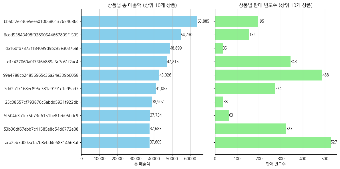
- 주문수와 매출액 추이는 비슷한 흐름으로 이루어져있음
- 총 매출액이 높다고 많이 팔리는 상품은 아닌것으로 관찰됐고, 해당 상품의 카테고리는 products데이터를 활용하면 확인할수있음
4. Products (olist_products_dataset.csv)
| 컬럼 이름 | 데이터 타입 | 설명 |
|---|---|---|
| product_id | VARCHAR | 상품 고유 식별자 |
| product_category_name | VARCHAR | 상품의 카테고리 이름 |
| product_name_length | INT | 상품 이름의 길이 |
| product_description_length | INT | 상품 설명의 길이 |
| product_photos_qty | INT | 상품 사진의 개수 |
| product_weight_g | FLOAT | 상품의 무게 (그램) |
| product_length_cm | FLOAT | 상품 길이 (센티미터) |
| product_height_cm | FLOAT | 상품 높이 (센티미터) |
| product_width_cm | FLOAT | 상품 폭 (센티미터) |
1
2
df4 = pd.read_csv('/content/drive/MyDrive/archive/olist_products_dataset.csv')
df4
| product_id | product_category_name | product_name_lenght | product_description_lenght | product_photos_qty | product_weight_g | product_length_cm | product_height_cm | product_width_cm | |
|---|---|---|---|---|---|---|---|---|---|
| 0 | 1e9e8ef04dbcff4541ed26657ea517e5 | perfumaria | 40.0 | 287.0 | 1.0 | 225.0 | 16.0 | 10.0 | 14.0 |
| 1 | 3aa071139cb16b67ca9e5dea641aaa2f | artes | 44.0 | 276.0 | 1.0 | 1000.0 | 30.0 | 18.0 | 20.0 |
| 2 | 96bd76ec8810374ed1b65e291975717f | esporte_lazer | 46.0 | 250.0 | 1.0 | 154.0 | 18.0 | 9.0 | 15.0 |
| 3 | cef67bcfe19066a932b7673e239eb23d | bebes | 27.0 | 261.0 | 1.0 | 371.0 | 26.0 | 4.0 | 26.0 |
| 4 | 9dc1a7de274444849c219cff195d0b71 | utilidades_domesticas | 37.0 | 402.0 | 4.0 | 625.0 | 20.0 | 17.0 | 13.0 |
| ... | ... | ... | ... | ... | ... | ... | ... | ... | ... |
| 32946 | a0b7d5a992ccda646f2d34e418fff5a0 | moveis_decoracao | 45.0 | 67.0 | 2.0 | 12300.0 | 40.0 | 40.0 | 40.0 |
| 32947 | bf4538d88321d0fd4412a93c974510e6 | construcao_ferramentas_iluminacao | 41.0 | 971.0 | 1.0 | 1700.0 | 16.0 | 19.0 | 16.0 |
| 32948 | 9a7c6041fa9592d9d9ef6cfe62a71f8c | cama_mesa_banho | 50.0 | 799.0 | 1.0 | 1400.0 | 27.0 | 7.0 | 27.0 |
| 32949 | 83808703fc0706a22e264b9d75f04a2e | informatica_acessorios | 60.0 | 156.0 | 2.0 | 700.0 | 31.0 | 13.0 | 20.0 |
| 32950 | 106392145fca363410d287a815be6de4 | cama_mesa_banho | 58.0 | 309.0 | 1.0 | 2083.0 | 12.0 | 2.0 | 7.0 |
32951 rows × 9 columns
1
2
# 결측치 찾기
df4.isna().sum().sort_values(ascending=False)
| 0 | |
|---|---|
| product_category_name | 610 |
| product_name_lenght | 610 |
| product_description_lenght | 610 |
| product_photos_qty | 610 |
| product_weight_g | 2 |
| product_length_cm | 2 |
| product_height_cm | 2 |
| product_width_cm | 2 |
| product_id | 0 |
1
2
mask1_df4 = df4[df4['product_category_name'].isna()]
df3[df3['product_id'].isin(mask1_df4['product_id'])]
| order_id | order_item_id | product_id | seller_id | shipping_limit_date | price | freight_value | |
|---|---|---|---|---|---|---|---|
| 123 | 0046e1d57f4c07c8c92ab26be8c3dfc0 | 1 | ff6caf9340512b8bf6d2a2a6df032cfa | 38e6dada03429a47197d5d584d793b41 | 2017-10-02 15:49:17 | 7.79 | 7.78 |
| 125 | 00482f2670787292280e0a8153d82467 | 1 | a9c404971d1a5b1cbc2e4070e02731fd | 702835e4b785b67a084280efca355756 | 2017-02-17 16:18:07 | 7.60 | 10.96 |
| 132 | 004f5d8f238e8908e6864b874eda3391 | 1 | 5a848e4ab52fd5445cdc07aab1c40e48 | c826c40d7b19f62a09e2d7c5e7295ee2 | 2018-03-06 09:29:25 | 122.99 | 15.61 |
| 142 | 0057199db02d1a5ef41bacbf41f8f63b | 1 | 41eee23c25f7a574dfaf8d5c151dbb12 | e5a3438891c0bfdb9394643f95273d8e | 2018-01-25 09:07:51 | 20.30 | 16.79 |
| 171 | 006cb7cafc99b29548d4f412c7f9f493 | 1 | e10758160da97891c2fdcbc35f0f031d | 323ce52b5b81df2cd804b017b7f09aa7 | 2018-02-22 13:35:28 | 56.00 | 14.14 |
| ... | ... | ... | ... | ... | ... | ... | ... |
| 112306 | ff24fec69b7f3d30f9dc1ab3aee7c179 | 1 | 5a848e4ab52fd5445cdc07aab1c40e48 | c826c40d7b19f62a09e2d7c5e7295ee2 | 2018-02-01 02:40:12 | 122.99 | 15.61 |
| 112333 | ff3024474be86400847879103757d1fd | 1 | f9b1795281ce51b1cf39ef6d101ae8ab | 3771c85bac139d2344864ede5d9341e3 | 2017-11-21 03:55:39 | 39.90 | 9.94 |
| 112350 | ff3a45ee744a7c1f8096d2e72c1a23e4 | 1 | b61d1388a17e3f547d2bc218df02335b | 07017df32dc5f2f1d2801e579548d620 | 2017-05-10 10:15:19 | 139.00 | 21.42 |
| 112438 | ff7b636282b98e0aa524264b295ed928 | 1 | 431df35e52c10451171d8037482eeb43 | 6cd68b3ed6d59aaa9fece558ad360c0a | 2018-02-22 15:35:35 | 49.90 | 15.11 |
| 112501 | ffa5e4c604dea4f0a59d19cc2322ac19 | 2 | bd421826916d3e1d445cb860cea3c0fb | 59cd88080b93f3c18508673122d26169 | 2017-12-11 08:41:20 | 29.99 | 15.10 |
1603 rows × 7 columns
1
2
mask2_df4 = df3[df3['product_id'].isin(mask1_df4['product_id'])]
df2[df2['order_id'].isin(mask2_df4['order_id'])]
| order_id | customer_id | order_status | order_purchase_timestamp | order_approved_at | order_delivered_carrier_date | order_delivered_customer_date | order_estimated_delivery_date | delivery_time | |
|---|---|---|---|---|---|---|---|---|---|
| 6 | 136cce7faa42fdb2cefd53fdc79a6098 | ed0271e0b7da060a393796590e7b737a | invoiced | 2017-04-11 12:22:08 | 2017-04-13 13:25:17 | NaN | NaT | 2017-05-09 00:00:00 | NaN |
| 107 | bfe42c22ecbf90bc9f35cf591270b6a7 | 803ac05904124294f8767894d6da532b | delivered | 2018-01-27 22:04:34 | 2018-01-27 22:16:18 | 2018-02-03 03:56:00 | 2018-02-09 20:16:40 | 2018-02-26 00:00:00 | 12.0 |
| 180 | 58ac1947c1a9067b9f416cba6d844a3f | ee8e1d37f563ecc11cc4dcb4dfd794c2 | delivered | 2017-09-13 09:18:50 | 2017-09-13 13:45:43 | 2017-09-14 21:20:03 | 2017-09-21 21:16:17 | 2017-09-25 00:00:00 | 8.0 |
| 228 | e22b71f6e4a481445ec4527cb4c405f7 | 1faf89c8f142db3fca6cf314c51a37b6 | delivered | 2017-04-22 13:48:18 | 2017-04-22 14:01:13 | 2017-04-24 19:08:53 | 2017-05-02 15:45:27 | 2017-05-11 00:00:00 | 10.0 |
| 263 | a094215e786240fcfefb83d18036a1cd | 86acfb656743da0c113d176832c9d535 | delivered | 2018-02-08 18:56:45 | 2018-02-08 19:32:18 | 2018-02-09 21:41:54 | 2018-02-19 13:28:50 | 2018-02-22 00:00:00 | 10.0 |
| ... | ... | ... | ... | ... | ... | ... | ... | ... | ... |
| 99069 | 1a10e938a1c7d8e5eecc3380f71ca76b | 8a81607347c25d881d995d94de6ad824 | delivered | 2018-07-25 08:58:35 | 2018-07-26 03:10:20 | 2018-07-27 11:32:00 | 2018-08-01 19:28:20 | 2018-08-10 00:00:00 | 7.0 |
| 99215 | e33865519137f5737444109ae8438633 | 64b086bdcc54458af3ea3bd838db54a5 | delivered | 2018-05-28 00:44:06 | 2018-05-29 03:31:17 | 2018-05-30 13:13:00 | 2018-06-01 22:25:39 | 2018-06-20 00:00:00 | 4.0 |
| 99222 | f0dd9af88d8ef5a8e4670fbbedaf19c4 | 30ddb50bd22ee927ebe308ea3da60735 | delivered | 2017-09-02 20:38:29 | 2017-09-05 04:24:12 | 2017-09-14 23:13:41 | 2017-09-15 14:59:50 | 2017-09-19 00:00:00 | 12.0 |
| 99228 | 272874573723eec18f23c0471927d778 | 48e080c8001e92ebea2b64e474f91a60 | delivered | 2017-12-20 23:10:33 | 2017-12-20 23:29:37 | 2017-12-21 21:49:35 | 2017-12-26 22:29:32 | 2018-01-09 00:00:00 | 5.0 |
| 99245 | dff2b9b8d7cfc595836945e1443789c3 | 2436fb2666a65fbacae82532e797cabf | delivered | 2018-07-16 12:59:02 | 2018-07-17 04:21:00 | 2018-07-17 15:08:00 | 2018-07-20 20:41:32 | 2018-08-07 00:00:00 | 4.0 |
1451 rows × 9 columns
- 상품이 카테고리화되지 않았지만 배송완료된 주문이 있다. 카테고리 미분류 상품으로 취급해야한다.
1
2
# 중복값 확인
df4['product_id'].duplicated().sum()
1
0
- products 데이터는 주문된 상품들의 정보를 보여주고있음
(참고) 상품명 번역 정보 (product_category_name_translation.csv)
1
2
df4_name = pd.read_csv('/content/drive/MyDrive/archive/product_category_name_translation.csv')
df4_name
| product_category_name | product_category_name_english | |
|---|---|---|
| 0 | beleza_saude | health_beauty |
| 1 | informatica_acessorios | computers_accessories |
| 2 | automotivo | auto |
| 3 | cama_mesa_banho | bed_bath_table |
| 4 | moveis_decoracao | furniture_decor |
| ... | ... | ... |
| 66 | flores | flowers |
| 67 | artes_e_artesanato | arts_and_craftmanship |
| 68 | fraldas_higiene | diapers_and_hygiene |
| 69 | fashion_roupa_infanto_juvenil | fashion_childrens_clothes |
| 70 | seguros_e_servicos | security_and_services |
71 rows × 2 columns
1
2
3
# 카테고리 영어로 변경
category_map = df4_name.set_index('product_category_name')['product_category_name_english'].to_dict()
df4['product_category_name'] = df4['product_category_name'].map(category_map).fillna(df4['product_category_name'])
1
df4['product_category_name'].unique()
1
2
3
4
5
6
7
8
9
10
11
12
13
14
15
16
17
18
19
20
21
22
23
24
25
26
27
array(['perfumery', 'art', 'sports_leisure', 'baby', 'housewares',
       'musical_instruments', 'cool_stuff', 'furniture_decor',
       'home_appliances', 'toys', 'bed_bath_table',
       'construction_tools_safety', 'computers_accessories',
       'health_beauty', 'luggage_accessories', 'garden_tools',
       'office_furniture', 'auto', 'electronics', 'fashion_shoes',
       'telephony', 'stationery', 'fashion_bags_accessories', 'computers',
       'home_construction', 'watches_gifts',
       'construction_tools_construction', 'pet_shop', 'small_appliances',
       'agro_industry_and_commerce', nan, 'furniture_living_room',
       'signaling_and_security', 'air_conditioning', 'consoles_games',
       'books_general_interest', 'costruction_tools_tools',
       'fashion_underwear_beach', 'fashion_male_clothing',
       'kitchen_dining_laundry_garden_furniture',
       'industry_commerce_and_business', 'fixed_telephony',
       'construction_tools_lights', 'books_technical',
       'home_appliances_2', 'party_supplies', 'drinks', 'market_place',
       'la_cuisine', 'costruction_tools_garden', 'fashio_female_clothing',
       'home_confort', 'audio', 'food_drink', 'music', 'food',
       'tablets_printing_image', 'books_imported',
       'small_appliances_home_oven_and_coffee', 'fashion_sport',
       'christmas_supplies', 'fashion_childrens_clothes', 'dvds_blu_ray',
       'arts_and_craftmanship', 'pc_gamer', 'furniture_bedroom',
       'cine_photo', 'diapers_and_hygiene', 'flowers', 'home_comfort_2',
       'portateis_cozinha_e_preparadores_de_alimentos',
       'security_and_services', 'furniture_mattress_and_upholstery',
       'cds_dvds_musicals'], dtype=object)
1
2
merged_df_product = pd.merge(df3, df4[['product_id', 'product_category_name']], on='product_id', how='left')
merged_df_product
| order_id | order_item_id | product_id | seller_id | shipping_limit_date | price | freight_value | product_category_name | |
|---|---|---|---|---|---|---|---|---|
| 0 | 00010242fe8c5a6d1ba2dd792cb16214 | 1 | 4244733e06e7ecb4970a6e2683c13e61 | 48436dade18ac8b2bce089ec2a041202 | 2017-09-19 09:45:35 | 58.90 | 13.29 | cool_stuff |
| 1 | 00018f77f2f0320c557190d7a144bdd3 | 1 | e5f2d52b802189ee658865ca93d83a8f | dd7ddc04e1b6c2c614352b383efe2d36 | 2017-05-03 11:05:13 | 239.90 | 19.93 | pet_shop |
| 2 | 000229ec398224ef6ca0657da4fc703e | 1 | c777355d18b72b67abbeef9df44fd0fd | 5b51032eddd242adc84c38acab88f23d | 2018-01-18 14:48:30 | 199.00 | 17.87 | furniture_decor |
| 3 | 00024acbcdf0a6daa1e931b038114c75 | 1 | 7634da152a4610f1595efa32f14722fc | 9d7a1d34a5052409006425275ba1c2b4 | 2018-08-15 10:10:18 | 12.99 | 12.79 | perfumery |
| 4 | 00042b26cf59d7ce69dfabb4e55b4fd9 | 1 | ac6c3623068f30de03045865e4e10089 | df560393f3a51e74553ab94004ba5c87 | 2017-02-13 13:57:51 | 199.90 | 18.14 | garden_tools |
| ... | ... | ... | ... | ... | ... | ... | ... | ... |
| 112645 | fffc94f6ce00a00581880bf54a75a037 | 1 | 4aa6014eceb682077f9dc4bffebc05b0 | b8bc237ba3788b23da09c0f1f3a3288c | 2018-05-02 04:11:01 | 299.99 | 43.41 | housewares |
| 112646 | fffcd46ef2263f404302a634eb57f7eb | 1 | 32e07fd915822b0765e448c4dd74c828 | f3c38ab652836d21de61fb8314b69182 | 2018-07-20 04:31:48 | 350.00 | 36.53 | computers_accessories |
| 112647 | fffce4705a9662cd70adb13d4a31832d | 1 | 72a30483855e2eafc67aee5dc2560482 | c3cfdc648177fdbbbb35635a37472c53 | 2017-10-30 17:14:25 | 99.90 | 16.95 | sports_leisure |
| 112648 | fffe18544ffabc95dfada21779c9644f | 1 | 9c422a519119dcad7575db5af1ba540e | 2b3e4a2a3ea8e01938cabda2a3e5cc79 | 2017-08-21 00:04:32 | 55.99 | 8.72 | computers_accessories |
| 112649 | fffe41c64501cc87c801fd61db3f6244 | 1 | 350688d9dc1e75ff97be326363655e01 | f7ccf836d21b2fb1de37564105216cc1 | 2018-06-12 17:10:13 | 43.00 | 12.79 | bed_bath_table |
112650 rows × 8 columns
1
2
3
4
5
6
7
8
9
10
11
12
13
14
15
16
17
18
19
20
21
22
23
24
25
26
27
28
29
30
31
32
33
34
35
36
37
38
39
40
41
42
43
44
45
46
47
48
49
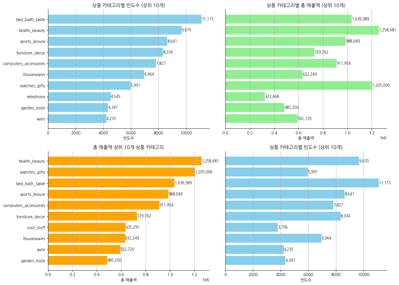
# 1. 'product_category_name'에 대한 빈도수 계산
category_counts = merged_df_product['product_category_name'].value_counts()
category_revenue = merged_df_product.groupby('product_category_name')['price'].sum()
# 2. 첫 번째 줄을 위한 상위 10개 카테고리 선택 및 정렬
top_categories_counts = category_counts.head(10).sort_values(ascending=True)
top_categories_revenue = category_revenue[top_categories_counts.index]
# 3. 두 번째 줄을 위한 총매출액 상위 10개 카테고리 선택 (정렬)
top_revenue_categories = category_revenue.nlargest(10).sort_values(ascending=True)
# 4. subplot 생성 (2x2)
fig, ((ax1, ax2), (ax3, ax4)) = plt.subplots(2, 2, figsize=(14, 10))
# 5. 차트 생성 함수
def create_bar_chart(ax, x_data, y_data, title, xlabel, color):
bars = ax.barh(x_data, y_data, color=color)
ax.set_title(title)
ax.set_xlabel(xlabel)
ax.grid(axis='x')
for bar in bars:
ax.text(bar.get_width(), bar.get_y() + bar.get_height()/2,
f'{bar.get_width():,.0f}', va='center', ha='left', fontsize=9)
# 6. 첫 번째 차트: 'product_category_name' 빈도수 (상위 10개)
create_bar_chart(ax1, top_categories_counts.index, top_categories_counts.values,
'상품 카테고리별 빈도수 (상위 10개)', '빈도수', 'skyblue')
# 7. 두 번째 차트: 'product_category_name'의 총 매출액 (상위 10개)
create_bar_chart(ax2, top_categories_counts.index, top_categories_revenue,
'상품 카테고리별 총 매출액 (상위 10개)', '총 매출액', 'lightgreen')
# 8. 세 번째 차트: 총매출액 상위 10개의 상품 카테고리
create_bar_chart(ax3, top_revenue_categories.index, top_revenue_categories.values,
'총 매출액 상위 10개 상품 카테고리', '총 매출액', 'orange')
# 9. 네 번째 차트: 빈도수 (상위 10개 카테고리, 정렬하지 않음)
create_bar_chart(ax4, top_revenue_categories.index, category_counts[top_revenue_categories.index],
'상품 카테고리별 빈도수 (상위 10개)', '빈도수', 'skyblue')
ax2.yaxis.set_visible(False)
ax4.yaxis.set_visible(False)
for ax in [ax1, ax2, ax3, ax4]:
ax.spines['top'].set_visible(False)
ax.spines['right'].set_visible(False)
plt.tight_layout()
plt.show()
1
2
3
4
5
6
7
8
9
10
11
12
13
14
15
16
17
18
19
20
21
22
23
24
25
26
27
28
29
30
31
32
33
34
35
36
37
38
39
40
41
42
43
44
45
46
47
48
49
50
51
52
53
54
55
56
57
58
# 1. 'product_category_name'에 대한 빈도수 계산
category_counts = merged_df_product['product_category_name'].value_counts()
category_revenue = merged_df_product.groupby('product_category_name')['price'].sum()

# 2. 전체 매출액 및 전체 빈도수 계산
total_revenue = category_revenue.sum()
total_count = category_counts.sum()

# 3. 첫 번째 줄을 위한 상위 10개 카테고리 선택 및 정렬
top_categories_counts = category_counts.head(10).sort_values(ascending=True)
top_categories_revenue = category_revenue[top_categories_counts.index]

# 4. 상위 10개 카테고리의 매출 비중 및 빈도 비중 계산
top_revenue_percentage = (top_categories_revenue / total_revenue) * 100
top_count_percentage = (top_categories_counts / total_count) * 100

# 5. subplot 생성 (2x2)
fig, ((ax1, ax2), (ax3, ax4)) = plt.subplots(2, 2, figsize=(14, 10))

# 6. 차트 생성 함수
def create_bar_chart(ax, x_data, y_data, title, xlabel, color):
    bars = ax.barh(x_data, y_data, color=color)
    ax.set_title(title)
    ax.set_xlabel(xlabel)
    ax.grid(axis='x')
    for bar in bars:
        ax.text(bar.get_width(), bar.get_y() + bar.get_height()/2,
                f'{bar.get_width():,.1f}%', va='center', ha='left', fontsize=9)

# 7. 첫 번째 차트: 'product_category_name' 빈도수 비중 (상위 10개)
create_bar_chart(ax1, top_categories_counts.index, top_count_percentage,
                 '상품 카테고리별 빈도수 비중 (%) (상위 10개)', '빈도수 비중 (%)', 'skyblue')

# 8. 두 번째 차트: 상위 10개 카테고리의 매출 비중
create_bar_chart(ax2, top_categories_counts.index, top_revenue_percentage,
                 '상품 카테고리별 매출 비중 (%) (상위 10개)', '매출 비중 (%)', 'lightgreen')

# 9. 세 번째 차트: 전체 매출액 상위 10개의 상품 카테고리 비중
top_revenue_categories = category_revenue.nlargest(10).sort_values(ascending=True)
top_revenue_categories_percentage = (top_revenue_categories / total_revenue) * 100
create_bar_chart(ax3, top_revenue_categories.index, top_revenue_categories_percentage,
                 '총 매출액 상위 10개 상품 카테고리 비중 (%)', '매출 비중 (%)', 'orange')

# 10. 네 번째 차트: 빈도수 (상위 10개 카테고리, 비중)
top_revenue_categories_counts = category_counts[top_revenue_categories.index]
top_revenue_categories_counts_percentage = (top_revenue_categories_counts / total_count) * 100
create_bar_chart(ax4, top_revenue_categories.index, top_revenue_categories_counts_percentage,
                 '상품 카테고리별 빈도수 비중 (%) (상위 10개)', '빈도수 비중 (%)', 'skyblue')

ax2.yaxis.set_visible(False)
ax4.yaxis.set_visible(False)

for ax in [ax1, ax2, ax3, ax4]:
    ax.spines['top'].set_visible(False)
    ax.spines['right'].set_visible(False)

plt.tight_layout()
plt.show()

- 판매량과 매출액이 반드시 비례하는것은 아닌것으로 관찰됨
- 특정 카테고리 매출비중이 높지않고 고르게 매출이 발생하고있으며, 건강과 미용 상품과 선물용 시계 상품이 각각 전체매출에 약 9% 비중을 차지하는 상위품목으로 관찰됨
5. Sellers (olist_sellers_dataset.csv)
| 컬럼 이름 | 데이터 타입 | 설명 |
|---|---|---|
| seller_id | VARCHAR | 판매자 고유 식별자 |
| seller_zip_code_prefix | INT | 판매자의 우편번호 앞부분 |
| seller_city | VARCHAR | 판매자의 도시 정보 |
| seller_state | VARCHAR | 판매자의 주 정보 |
1
2
df5 = pd.read_csv('/content/drive/MyDrive/archive/olist_sellers_dataset.csv')
df5
| seller_id | seller_zip_code_prefix | seller_city | seller_state | |
|---|---|---|---|---|
| 0 | 3442f8959a84dea7ee197c632cb2df15 | 13023 | campinas | SP |
| 1 | d1b65fc7debc3361ea86b5f14c68d2e2 | 13844 | mogi guacu | SP |
| 2 | ce3ad9de960102d0677a81f5d0bb7b2d | 20031 | rio de janeiro | RJ |
| 3 | c0f3eea2e14555b6faeea3dd58c1b1c3 | 4195 | sao paulo | SP |
| 4 | 51a04a8a6bdcb23deccc82b0b80742cf | 12914 | braganca paulista | SP |
| ... | ... | ... | ... | ... |
| 3090 | 98dddbc4601dd4443ca174359b237166 | 87111 | sarandi | PR |
| 3091 | f8201cab383e484733266d1906e2fdfa | 88137 | palhoca | SC |
| 3092 | 74871d19219c7d518d0090283e03c137 | 4650 | sao paulo | SP |
| 3093 | e603cf3fec55f8697c9059638d6c8eb5 | 96080 | pelotas | RS |
| 3094 | 9e25199f6ef7e7c347120ff175652c3b | 12051 | taubate | SP |
3095 rows × 4 columns
1
2
# 결측치 확인
df5.isna().sum().sort_values(ascending=False)
| 0 | |
|---|---|
| seller_id | 0 |
| seller_zip_code_prefix | 0 |
| seller_city | 0 |
| seller_state | 0 |
1
2
# 중복값 확인
df5['seller_id'].duplicated().sum()
1
0
- sellers 데이터는 olist에서 판매중인 고객 정보를 담고있으며, 총 3,095명 고객이 판매를 하고있다
1
2
3
4
df3_new = df3.copy()
df3_new = df3_new.merge(df2, on='order_id', how='left')
df3_new = df3_new.merge(df, on='customer_id', how='left')
df3_new = df3_new.merge(df5, on='seller_id', how='left')
1
df3_new
| order_id | order_item_id | product_id | seller_id | shipping_limit_date | price | freight_value | customer_id | order_status | order_purchase_timestamp | ... | order_delivered_customer_date | order_estimated_delivery_date | delivery_time | customer_unique_id | customer_zip_code_prefix | customer_city | customer_state | seller_zip_code_prefix | seller_city | seller_state | |
|---|---|---|---|---|---|---|---|---|---|---|---|---|---|---|---|---|---|---|---|---|---|
| 0 | 00010242fe8c5a6d1ba2dd792cb16214 | 1 | 4244733e06e7ecb4970a6e2683c13e61 | 48436dade18ac8b2bce089ec2a041202 | 2017-09-19 09:45:35 | 58.90 | 13.29 | 3ce436f183e68e07877b285a838db11a | delivered | 2017-09-13 08:59:02 | ... | 2017-09-20 23:43:48 | 2017-09-29 00:00:00 | 7.0 | 871766c5855e863f6eccc05f988b23cb | 28013 | campos dos goytacazes | RJ | 27277 | volta redonda | SP |
| 1 | 00018f77f2f0320c557190d7a144bdd3 | 1 | e5f2d52b802189ee658865ca93d83a8f | dd7ddc04e1b6c2c614352b383efe2d36 | 2017-05-03 11:05:13 | 239.90 | 19.93 | f6dd3ec061db4e3987629fe6b26e5cce | delivered | 2017-04-26 10:53:06 | ... | 2017-05-12 16:04:24 | 2017-05-15 00:00:00 | 16.0 | eb28e67c4c0b83846050ddfb8a35d051 | 15775 | santa fe do sul | SP | 3471 | sao paulo | SP |
| 2 | 000229ec398224ef6ca0657da4fc703e | 1 | c777355d18b72b67abbeef9df44fd0fd | 5b51032eddd242adc84c38acab88f23d | 2018-01-18 14:48:30 | 199.00 | 17.87 | 6489ae5e4333f3693df5ad4372dab6d3 | delivered | 2018-01-14 14:33:31 | ... | 2018-01-22 13:19:16 | 2018-02-05 00:00:00 | 7.0 | 3818d81c6709e39d06b2738a8d3a2474 | 35661 | para de minas | MG | 37564 | borda da mata | MG |
| 3 | 00024acbcdf0a6daa1e931b038114c75 | 1 | 7634da152a4610f1595efa32f14722fc | 9d7a1d34a5052409006425275ba1c2b4 | 2018-08-15 10:10:18 | 12.99 | 12.79 | d4eb9395c8c0431ee92fce09860c5a06 | delivered | 2018-08-08 10:00:35 | ... | 2018-08-14 13:32:39 | 2018-08-20 00:00:00 | 6.0 | af861d436cfc08b2c2ddefd0ba074622 | 12952 | atibaia | SP | 14403 | franca | SP |
| 4 | 00042b26cf59d7ce69dfabb4e55b4fd9 | 1 | ac6c3623068f30de03045865e4e10089 | df560393f3a51e74553ab94004ba5c87 | 2017-02-13 13:57:51 | 199.90 | 18.14 | 58dbd0b2d70206bf40e62cd34e84d795 | delivered | 2017-02-04 13:57:51 | ... | 2017-03-01 16:42:31 | 2017-03-17 00:00:00 | 25.0 | 64b576fb70d441e8f1b2d7d446e483c5 | 13226 | varzea paulista | SP | 87900 | loanda | PR |
| ... | ... | ... | ... | ... | ... | ... | ... | ... | ... | ... | ... | ... | ... | ... | ... | ... | ... | ... | ... | ... | ... |
| 112645 | fffc94f6ce00a00581880bf54a75a037 | 1 | 4aa6014eceb682077f9dc4bffebc05b0 | b8bc237ba3788b23da09c0f1f3a3288c | 2018-05-02 04:11:01 | 299.99 | 43.41 | b51593916b4b8e0d6f66f2ae24f2673d | delivered | 2018-04-23 13:57:06 | ... | 2018-05-10 22:56:40 | 2018-05-18 00:00:00 | 17.0 | 0c9aeda10a71f369396d0c04dce13a64 | 65077 | sao luis | MA | 88303 | itajai | SC |
| 112646 | fffcd46ef2263f404302a634eb57f7eb | 1 | 32e07fd915822b0765e448c4dd74c828 | f3c38ab652836d21de61fb8314b69182 | 2018-07-20 04:31:48 | 350.00 | 36.53 | 84c5d4fbaf120aae381fad077416eaa0 | delivered | 2018-07-14 10:26:46 | ... | 2018-07-23 20:31:55 | 2018-08-01 00:00:00 | 9.0 | 0da9fe112eae0c74d3ba1fe16de0988b | 81690 | curitiba | PR | 1206 | sao paulo | SP |
| 112647 | fffce4705a9662cd70adb13d4a31832d | 1 | 72a30483855e2eafc67aee5dc2560482 | c3cfdc648177fdbbbb35635a37472c53 | 2017-10-30 17:14:25 | 99.90 | 16.95 | 29309aa813182aaddc9b259e31b870e6 | delivered | 2017-10-23 17:07:56 | ... | 2017-10-28 12:22:22 | 2017-11-10 00:00:00 | 4.0 | cd79b407828f02fdbba457111c38e4c4 | 4039 | sao paulo | SP | 80610 | curitiba | PR |
| 112648 | fffe18544ffabc95dfada21779c9644f | 1 | 9c422a519119dcad7575db5af1ba540e | 2b3e4a2a3ea8e01938cabda2a3e5cc79 | 2017-08-21 00:04:32 | 55.99 | 8.72 | b5e6afd5a41800fdf401e0272ca74655 | delivered | 2017-08-14 23:02:59 | ... | 2017-08-16 21:59:40 | 2017-08-25 00:00:00 | 1.0 | eb803377c9315b564bdedad672039306 | 13289 | vinhedo | SP | 4733 | sao paulo | SP |
| 112649 | fffe41c64501cc87c801fd61db3f6244 | 1 | 350688d9dc1e75ff97be326363655e01 | f7ccf836d21b2fb1de37564105216cc1 | 2018-06-12 17:10:13 | 43.00 | 12.79 | 96d649da0cc4ff33bb408b199d4c7dcf | delivered | 2018-06-09 17:00:18 | ... | 2018-06-14 17:56:26 | 2018-06-28 00:00:00 | 5.0 | cd76a00d8e3ca5e6ab9ed9ecb6667ac4 | 18605 | botucatu | SP | 14940 | ibitinga | SP |
112650 rows × 22 columns
1
2
3
4
5
6
7
8
9
10
11
12
13
14
15
16
17
18
19
20
21
22
23
24
25
26
27
28
29
30
31
32
33
34
35
# 1. customer_state와 seller_state의 빈도수 계산
customer_state_counts = df3_new['customer_state'].value_counts().head(10).sort_values(ascending=True)
seller_state_counts = df3_new['seller_state'].value_counts().head(10).sort_values(ascending=True)

# 2. subplot 생성 (1x2)
fig, (ax1, ax2) = plt.subplots(1, 2, figsize=(14, 6))

# 3. 첫 번째 차트: customer_state 빈도수
bars1 = ax1.barh(customer_state_counts.index, customer_state_counts.values, color='skyblue')
ax1.set_title('상위 10개 고객 주(State) 빈도수')
ax1.set_xlabel('빈도수')
ax1.grid(axis='x')

# 4. 숫자 표기
for bar in bars1:
    ax1.text(bar.get_width(), bar.get_y() + bar.get_height()/2,
             f'{bar.get_width():,.0f}', va='center', ha='left', fontsize=9)

# 5. 두 번째 차트: seller_state 빈도수
bars2 = ax2.barh(seller_state_counts.index, seller_state_counts.values, color='lightgreen')
ax2.set_title('상위 10개 판매자 주(State) 빈도수')
ax2.set_xlabel('빈도수')
ax2.grid(axis='x')

for bar in bars2:
    ax2.text(bar.get_width(), bar.get_y() + bar.get_height()/2,
             f'{bar.get_width():,.0f}', va='center', ha='left', fontsize=9)

ax1.spines['top'].set_visible(False)
ax1.spines['right'].set_visible(False)
ax2.spines['top'].set_visible(False)
ax2.spines['right'].set_visible(False)

plt.tight_layout()
plt.show()
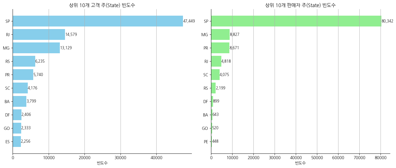
- 대부분의 상품은 SP주에서 배송되고있으며, 구매 고객과 판매 고객의 위치 차이로 배송기간이 길어질 수 있음
6. Order Payments (olist_order_payments_dataset.csv)
| 컬럼 이름 | 데이터 타입 | 설명 |
|---|---|---|
| order_id | VARCHAR | 주문 고유 식별자 |
| payment_sequential | INT | 각 주문의 결제 수단 순서 |
| payment_type | VARCHAR | 결제 방식 (신용카드, 현금 등) |
| payment_installments | INT | 할부 개월 수 |
| payment_value | FLOAT | 결제 금액 |
1
2
df6 = pd.read_csv('/content/drive/MyDrive/archive/olist_order_payments_dataset.csv')
df6
| order_id | payment_sequential | payment_type | payment_installments | payment_value | |
|---|---|---|---|---|---|
| 0 | b81ef226f3fe1789b1e8b2acac839d17 | 1 | credit_card | 8 | 99.33 |
| 1 | a9810da82917af2d9aefd1278f1dcfa0 | 1 | credit_card | 1 | 24.39 |
| 2 | 25e8ea4e93396b6fa0d3dd708e76c1bd | 1 | credit_card | 1 | 65.71 |
| 3 | ba78997921bbcdc1373bb41e913ab953 | 1 | credit_card | 8 | 107.78 |
| 4 | 42fdf880ba16b47b59251dd489d4441a | 1 | credit_card | 2 | 128.45 |
| ... | ... | ... | ... | ... | ... |
| 103881 | 0406037ad97740d563a178ecc7a2075c | 1 | boleto | 1 | 363.31 |
| 103882 | 7b905861d7c825891d6347454ea7863f | 1 | credit_card | 2 | 96.80 |
| 103883 | 32609bbb3dd69b3c066a6860554a77bf | 1 | credit_card | 1 | 47.77 |
| 103884 | b8b61059626efa996a60be9bb9320e10 | 1 | credit_card | 5 | 369.54 |
| 103885 | 28bbae6599b09d39ca406b747b6632b1 | 1 | boleto | 1 | 191.58 |
103886 rows × 5 columns
1
2
# 결측치 확인
df6.isna().sum().sort_values(ascending=False)
| 0 | |
|---|---|
| order_id | 0 |
| payment_sequential | 0 |
| payment_type | 0 |
| payment_installments | 0 |
| payment_value | 0 |
1
2
# 중복값 확인
df6['order_id'].duplicated().sum()
1
4446
1
df6['payment_sequential'].value_counts()
| count | |
|---|---|
| payment_sequential | |
| 1 | 99360 |
| 2 | 3039 |
| 3 | 581 |
| 4 | 278 |
| 5 | 170 |
| 6 | 118 |
| 7 | 82 |
| 8 | 54 |
| 9 | 43 |
| 10 | 34 |
| 11 | 29 |
| 12 | 21 |
| 13 | 13 |
| 14 | 10 |
| 15 | 8 |
| 18 | 6 |
| 19 | 6 |
| 16 | 6 |
| 17 | 6 |
| 21 | 4 |
| 20 | 4 |
| 22 | 3 |
| 26 | 2 |
| 24 | 2 |
| 23 | 2 |
| 25 | 2 |
| 29 | 1 |
| 28 | 1 |
| 27 | 1 |
1
df6['payment_installments'].value_counts()
| count | |
|---|---|
| payment_installments | |
| 1 | 52546 |
| 2 | 12413 |
| 3 | 10461 |
| 4 | 7098 |
| 10 | 5328 |
| 5 | 5239 |
| 8 | 4268 |
| 6 | 3920 |
| 7 | 1626 |
| 9 | 644 |
| 12 | 133 |
| 15 | 74 |
| 18 | 27 |
| 11 | 23 |
| 24 | 18 |
| 20 | 17 |
| 13 | 16 |
| 14 | 15 |
| 17 | 8 |
| 16 | 5 |
| 21 | 3 |
| 0 | 2 |
| 22 | 1 |
| 23 | 1 |
1
round((df6[df6['payment_installments'] >= 6].shape[0] / df6.shape[0]) * 100, 2)
1
15.52
1
df6['payment_type'].value_counts()
| count | |
|---|---|
| payment_type | |
| credit_card | 76795 |
| boleto | 19784 |
| voucher | 5775 |
| debit_card | 1529 |
| not_defined | 3 |
1
round((df6[df6['payment_type'] == 'boleto'].shape[0] / df6.shape[0])*100, 2)
1
19.04
- 주문별 결제수단을 1번혹은 여러번 사용
- order 데이터의 order_id보다 주문수가 적은것을 보아 취소나 변경 등 주문후 결제정보가 삭제된 데이터들이 존재함
- 6개월 이상 장기 할부 거래가 15% 정도 발생하고 있음(boleto 거래 포함시 약 34%)
7. Order Reviews (olist_order_reviews_dataset.csv)
| 컬럼 이름 | 데이터 타입 | 설명 |
|---|---|---|
| review_id | VARCHAR | 리뷰 고유 식별자 |
| order_id | VARCHAR | 리뷰와 연결된 주문 고유 식별자 |
| review_score | INT | 고객이 남긴 평점 |
| review_comment_title | VARCHAR | 리뷰 제목 |
| review_comment_message | TEXT | 리뷰 내용 |
| review_creation_date | TIMESTAMP | 리뷰가 생성된 날짜 |
| review_answer_timestamp | TIMESTAMP | 리뷰에 답변한 시각 |
1
2
df7 = pd.read_csv('/content/drive/MyDrive/archive/olist_order_reviews_dataset.csv')
df7
| review_id | order_id | review_score | review_comment_title | review_comment_message | review_creation_date | review_answer_timestamp | |
|---|---|---|---|---|---|---|---|
| 0 | 7bc2406110b926393aa56f80a40eba40 | 73fc7af87114b39712e6da79b0a377eb | 4 | NaN | NaN | 2018-01-18 00:00:00 | 2018-01-18 21:46:59 |
| 1 | 80e641a11e56f04c1ad469d5645fdfde | a548910a1c6147796b98fdf73dbeba33 | 5 | NaN | NaN | 2018-03-10 00:00:00 | 2018-03-11 03:05:13 |
| 2 | 228ce5500dc1d8e020d8d1322874b6f0 | f9e4b658b201a9f2ecdecbb34bed034b | 5 | NaN | NaN | 2018-02-17 00:00:00 | 2018-02-18 14:36:24 |
| 3 | e64fb393e7b32834bb789ff8bb30750e | 658677c97b385a9be170737859d3511b | 5 | NaN | Recebi bem antes do prazo estipulado. | 2017-04-21 00:00:00 | 2017-04-21 22:02:06 |
| 4 | f7c4243c7fe1938f181bec41a392bdeb | 8e6bfb81e283fa7e4f11123a3fb894f1 | 5 | NaN | Parabéns lojas lannister adorei comprar pela I... | 2018-03-01 00:00:00 | 2018-03-02 10:26:53 |
| ... | ... | ... | ... | ... | ... | ... | ... |
| 99219 | 574ed12dd733e5fa530cfd4bbf39d7c9 | 2a8c23fee101d4d5662fa670396eb8da | 5 | NaN | NaN | 2018-07-07 00:00:00 | 2018-07-14 17:18:30 |
| 99220 | f3897127253a9592a73be9bdfdf4ed7a | 22ec9f0669f784db00fa86d035cf8602 | 5 | NaN | NaN | 2017-12-09 00:00:00 | 2017-12-11 20:06:42 |
| 99221 | b3de70c89b1510c4cd3d0649fd302472 | 55d4004744368f5571d1f590031933e4 | 5 | NaN | Excelente mochila, entrega super rápida. Super... | 2018-03-22 00:00:00 | 2018-03-23 09:10:43 |
| 99222 | 1adeb9d84d72fe4e337617733eb85149 | 7725825d039fc1f0ceb7635e3f7d9206 | 4 | NaN | NaN | 2018-07-01 00:00:00 | 2018-07-02 12:59:13 |
| 99223 | efe49f1d6f951dd88b51e6ccd4cc548f | 90531360ecb1eec2a1fbb265a0db0508 | 1 | NaN | meu produto chegou e ja tenho que devolver, po... | 2017-07-03 00:00:00 | 2017-07-03 21:01:49 |
99224 rows × 7 columns
1
2
# 결측치 확인
df7.isna().sum().sort_values(ascending=False)
| 0 | |
|---|---|
| review_comment_title | 87656 |
| review_comment_message | 58247 |
| review_id | 0 |
| order_id | 0 |
| review_score | 0 |
| review_creation_date | 0 |
| review_answer_timestamp | 0 |
- 리뷰를 안적는사람이 있기때문에 결측치가 아님
1
2
3
# 중복값 확인
print(df7['order_id'].duplicated().sum())
print(df7['review_id'].duplicated().sum())
1
2
551
814
1
df7[df7['order_id'].duplicated(keep=False)].sort_values(by=['order_id'])
| review_id | order_id | review_score | review_comment_title | review_comment_message | review_creation_date | review_answer_timestamp | |
|---|---|---|---|---|---|---|---|
| 25612 | 89a02c45c340aeeb1354a24e7d4b2c1e | 0035246a40f520710769010f752e7507 | 5 | NaN | NaN | 2017-08-29 00:00:00 | 2017-08-30 01:59:12 |
| 22423 | 2a74b0559eb58fc1ff842ecc999594cb | 0035246a40f520710769010f752e7507 | 5 | NaN | Estou acostumada a comprar produtos pelo barat... | 2017-08-25 00:00:00 | 2017-08-29 21:45:57 |
| 22779 | ab30810c29da5da8045216f0f62652a2 | 013056cfe49763c6f66bda03396c5ee3 | 5 | NaN | NaN | 2018-02-22 00:00:00 | 2018-02-23 12:12:30 |
| 68633 | 73413b847f63e02bc752b364f6d05ee9 | 013056cfe49763c6f66bda03396c5ee3 | 4 | NaN | NaN | 2018-03-04 00:00:00 | 2018-03-05 17:02:00 |
| 854 | 830636803620cdf8b6ffaf1b2f6e92b2 | 0176a6846bcb3b0d3aa3116a9a768597 | 5 | NaN | NaN | 2017-12-30 00:00:00 | 2018-01-02 10:54:06 |
| ... | ... | ... | ... | ... | ... | ... | ... |
| 27465 | 5e78482ee783451be6026e5cf0c72de1 | ff763b73e473d03c321bcd5a053316e8 | 3 | NaN | Não sei que haverá acontecido os demais chegaram | 2017-11-18 00:00:00 | 2017-11-18 09:02:48 |
| 41355 | 39de8ad3a1a494fc68cc2d5382f052f4 | ff850ba359507b996e8b2fbb26df8d03 | 5 | NaN | Envio rapido... Produto 100% | 2017-08-16 00:00:00 | 2017-08-17 11:56:55 |
| 18783 | 80f25f32c00540d49d57796fb6658535 | ff850ba359507b996e8b2fbb26df8d03 | 5 | NaN | Envio rapido, produto conforme descrito no anu... | 2017-08-22 00:00:00 | 2017-08-25 11:40:22 |
| 92230 | 870d856a4873d3a67252b0c51d79b950 | ffaabba06c9d293a3c614e0515ddbabc | 3 | NaN | NaN | 2017-12-20 00:00:00 | 2017-12-20 18:50:16 |
| 53962 | 5476dd0eaee7c4e2725cafb011aa758c | ffaabba06c9d293a3c614e0515ddbabc | 3 | NaN | NaN | 2017-12-20 00:00:00 | 2017-12-21 13:24:55 |
1098 rows × 7 columns
1
df7[df7['order_id'] == 'ff850ba359507b996e8b2fbb26df8d03']
| review_id | order_id | review_score | review_comment_title | review_comment_message | review_creation_date | review_answer_timestamp | |
|---|---|---|---|---|---|---|---|
| 18783 | 80f25f32c00540d49d57796fb6658535 | ff850ba359507b996e8b2fbb26df8d03 | 5 | NaN | Envio rapido, produto conforme descrito no anu... | 2017-08-22 00:00:00 | 2017-08-25 11:40:22 |
| 41355 | 39de8ad3a1a494fc68cc2d5382f052f4 | ff850ba359507b996e8b2fbb26df8d03 | 5 | NaN | Envio rapido... Produto 100% | 2017-08-16 00:00:00 | 2017-08-17 11:56:55 |
1
df3[df3['order_id'] == 'ff850ba359507b996e8b2fbb26df8d03']
| order_id | order_item_id | product_id | seller_id | shipping_limit_date | price | freight_value | |
|---|---|---|---|---|---|---|---|
| 112446 | ff850ba359507b996e8b2fbb26df8d03 | 1 | d2bea3c01e172037caa99b2d138f39d0 | 9674754b5a0cb32b638cec001178f799 | 2017-08-10 20:20:07 | 16.9 | 16.11 |
1
df6[df6['order_id'] == 'ff850ba359507b996e8b2fbb26df8d03']
| order_id | payment_sequential | payment_type | payment_installments | payment_value | |
|---|---|---|---|---|---|
| 8576 | ff850ba359507b996e8b2fbb26df8d03 | 1 | credit_card | 3 | 33.01 |
1
df2[df2['order_id'] == 'ff850ba359507b996e8b2fbb26df8d03']
| order_id | customer_id | order_status | order_purchase_timestamp | order_approved_at | order_delivered_carrier_date | order_delivered_customer_date | order_estimated_delivery_date | delivery_time | |
|---|---|---|---|---|---|---|---|---|---|
| 68231 | ff850ba359507b996e8b2fbb26df8d03 | 219399e5496f8ca1dc6f68753131c084 | delivered | 2017-08-06 19:38:00 | 2017-08-06 20:20:07 | 2017-08-08 12:23:16 | 2017-08-21 22:15:41 | 2017-08-31 00:00:00 | 15.0 |
- 해당주문번호로 리뷰를 2번썼는데, 첫번째는 도착하기도전에 리뷰가 적혔다
1
df7.groupby('order_id').filter(lambda x: len(x) >= 3)
| review_id | order_id | review_score | review_comment_title | review_comment_message | review_creation_date | review_answer_timestamp | |
|---|---|---|---|---|---|---|---|
| 1985 | ffb8cff872a625632ac983eb1f88843c | c88b1d1b157a9999ce368f218a407141 | 3 | NaN | NaN | 2017-07-22 00:00:00 | 2017-07-26 13:41:07 |
| 2952 | c444278834184f72b1484dfe47de7f97 | df56136b8031ecd28e200bb18e6ddb2e | 5 | NaN | NaN | 2017-02-08 00:00:00 | 2017-02-14 13:58:48 |
| 8273 | b04ed893318da5b863e878cd3d0511df | 03c939fd7fd3b38f8485a0f95798f1f6 | 3 | NaN | Um ponto negativo que achei foi a cobrança de ... | 2018-03-20 00:00:00 | 2018-03-21 02:28:23 |
| 13982 | 72a1098d5b410ae50fbc0509d26daeb9 | df56136b8031ecd28e200bb18e6ddb2e | 5 | NaN | NaN | 2017-02-07 00:00:00 | 2017-02-10 10:46:09 |
| 44694 | 67c2557eb0bd72e3ece1e03477c9dff5 | 8e17072ec97ce29f0e1f111e598b0c85 | 1 | NaN | Entregou o produto errado. | 2018-04-07 00:00:00 | 2018-04-08 22:48:27 |
| 51527 | f4bb9d6dd4fb6dcc2298f0e7b17b8e1e | 03c939fd7fd3b38f8485a0f95798f1f6 | 4 | NaN | NaN | 2018-03-29 00:00:00 | 2018-03-30 00:29:09 |
| 62728 | 44f3e54834d23c5570c1d010824d4d59 | df56136b8031ecd28e200bb18e6ddb2e | 5 | NaN | NaN | 2017-02-09 00:00:00 | 2017-02-09 09:07:28 |
| 64510 | 2d6ac45f859465b5c185274a1c929637 | 8e17072ec97ce29f0e1f111e598b0c85 | 1 | NaN | Comprei 3 unidades do produto vieram 2 unidade... | 2018-04-07 00:00:00 | 2018-04-07 21:13:05 |
| 69438 | 405eb2ea45e1dbe2662541ae5b47e2aa | 03c939fd7fd3b38f8485a0f95798f1f6 | 3 | NaN | Seria ótimo se tivesem entregue os 3 (três) pe... | 2018-03-06 00:00:00 | 2018-03-06 19:50:32 |
| 82525 | 202b5f44d09cd3cfc0d6bd12f01b044c | c88b1d1b157a9999ce368f218a407141 | 5 | NaN | NaN | 2017-07-22 00:00:00 | 2017-07-26 13:40:22 |
| 89360 | fb96ea2ef8cce1c888f4d45c8e22b793 | c88b1d1b157a9999ce368f218a407141 | 5 | NaN | NaN | 2017-07-21 00:00:00 | 2017-07-26 13:45:15 |
| 92300 | 6e4c4086d9611ae4cc0cc65a262751fe | 8e17072ec97ce29f0e1f111e598b0c85 | 1 | NaN | Embora tenha entregue dentro do prazo, não env... | 2018-04-14 00:00:00 | 2018-04-16 11:37:31 |
1
df7[df7['order_id'] == 'c88b1d1b157a9999ce368f218a407141']
| review_id | order_id | review_score | review_comment_title | review_comment_message | review_creation_date | review_answer_timestamp | |
|---|---|---|---|---|---|---|---|
| 1985 | ffb8cff872a625632ac983eb1f88843c | c88b1d1b157a9999ce368f218a407141 | 3 | NaN | NaN | 2017-07-22 00:00:00 | 2017-07-26 13:41:07 |
| 82525 | 202b5f44d09cd3cfc0d6bd12f01b044c | c88b1d1b157a9999ce368f218a407141 | 5 | NaN | NaN | 2017-07-22 00:00:00 | 2017-07-26 13:40:22 |
| 89360 | fb96ea2ef8cce1c888f4d45c8e22b793 | c88b1d1b157a9999ce368f218a407141 | 5 | NaN | NaN | 2017-07-21 00:00:00 | 2017-07-26 13:45:15 |
1
df3[df3['order_id'] == 'c88b1d1b157a9999ce368f218a407141']
| order_id | order_item_id | product_id | seller_id | shipping_limit_date | price | freight_value | |
|---|---|---|---|---|---|---|---|
| 88316 | c88b1d1b157a9999ce368f218a407141 | 1 | b1acb7e8152c90c9619897753a75c973 | cc419e0650a3c5ba77189a1882b7556a | 2017-07-26 22:50:12 | 34.99 | 7.78 |
1
df6[df6['order_id'] == 'c88b1d1b157a9999ce368f218a407141']
| order_id | payment_sequential | payment_type | payment_installments | payment_value | |
|---|---|---|---|---|---|
| 103471 | c88b1d1b157a9999ce368f218a407141 | 1 | credit_card | 4 | 42.77 |
1
df7[df7['review_id'].duplicated(keep=False)].sort_values(by=['review_id']).head(30)
| review_id | order_id | review_score | review_comment_title | review_comment_message | review_creation_date | review_answer_timestamp | |
|---|---|---|---|---|---|---|---|
| 46678 | 00130cbe1f9d422698c812ed8ded1919 | dfcdfc43867d1c1381bfaf62d6b9c195 | 1 | NaN | O cartucho "original HP" 60XL não é reconhecid... | 2018-03-07 00:00:00 | 2018-03-20 18:08:23 |
| 29841 | 00130cbe1f9d422698c812ed8ded1919 | 04a28263e085d399c97ae49e0b477efa | 1 | NaN | O cartucho "original HP" 60XL não é reconhecid... | 2018-03-07 00:00:00 | 2018-03-20 18:08:23 |
| 90677 | 0115633a9c298b6a98bcbe4eee75345f | 78a4201f58af3463bdab842eea4bc801 | 5 | NaN | NaN | 2017-09-21 00:00:00 | 2017-09-26 03:27:47 |
| 63193 | 0115633a9c298b6a98bcbe4eee75345f | 0c9850b2c179c1ef60d2855e2751d1fa | 5 | NaN | NaN | 2017-09-21 00:00:00 | 2017-09-26 03:27:47 |
| 92876 | 0174caf0ee5964646040cd94e15ac95e | f93a732712407c02dce5dd5088d0f47b | 1 | NaN | Produto entregue dentro de embalagem do fornec... | 2018-03-07 00:00:00 | 2018-03-08 03:00:53 |
| 57280 | 0174caf0ee5964646040cd94e15ac95e | 74db91e33b4e1fd865356c89a61abf1f | 1 | NaN | Produto entregue dentro de embalagem do fornec... | 2018-03-07 00:00:00 | 2018-03-08 03:00:53 |
| 54832 | 017808d29fd1f942d97e50184dfb4c13 | 8daaa9e99d60fbba579cc1c3e3bfae01 | 5 | NaN | NaN | 2018-03-02 00:00:00 | 2018-03-05 01:43:30 |
| 99167 | 017808d29fd1f942d97e50184dfb4c13 | b1461c8882153b5fe68307c46a506e39 | 5 | NaN | NaN | 2018-03-02 00:00:00 | 2018-03-05 01:43:30 |
| 20621 | 0254bd905dc677a6078990aad3331a36 | 5bf226cf882c5bf4247f89a97c86f273 | 1 | NaN | O pedido consta de 2 produtos e até agora rece... | 2017-09-09 00:00:00 | 2017-09-13 09:52:44 |
| 96080 | 0254bd905dc677a6078990aad3331a36 | 331b367bdd766f3d1cf518777317b5d9 | 1 | NaN | O pedido consta de 2 produtos e até agora rece... | 2017-09-09 00:00:00 | 2017-09-13 09:52:44 |
| 89712 | 0288d42bef3dfe36930740c9588a570f | 33d8795f04dd631f3480d7aaf90da3dc | 3 | NaN | NaN | 2017-07-29 00:00:00 | 2017-07-31 17:11:04 |
| 94851 | 0288d42bef3dfe36930740c9588a570f | f889a5a0b44adc29c5465b99395ac3c1 | 3 | NaN | NaN | 2017-07-29 00:00:00 | 2017-07-31 17:11:04 |
| 47495 | 02aa7f5f75e964e3c7efa59a1f515281 | d8e17d5f7dacf0970d316e7c03e741e8 | 3 | NaN | NaN | 2017-07-27 00:00:00 | 2017-07-29 15:09:50 |
| 95860 | 02aa7f5f75e964e3c7efa59a1f515281 | db92613c074f00e53066388d48ad7512 | 3 | NaN | NaN | 2017-07-27 00:00:00 | 2017-07-29 15:09:50 |
| 71165 | 034528cb00b6bc981847acafbdf2ae0b | e1e8e3bca903de27e9a1c72b5a5795e0 | 1 | NaN | NaN | 2017-05-14 00:00:00 | 2017-05-15 02:17:38 |
| 81094 | 034528cb00b6bc981847acafbdf2ae0b | 3d3742a96f24a8fe4e2e57628807e476 | 1 | NaN | NaN | 2017-05-14 00:00:00 | 2017-05-15 02:17:38 |
| 1988 | 03a6a25db577d0689440933055111897 | 2acfdc5131ff2cf4433e668454c9784c | 5 | NaN | Muito Bom! Gostei Bastante! Tecido Ótimo! Aten... | 2017-12-15 00:00:00 | 2017-12-16 01:32:18 |
| 9013 | 03a6a25db577d0689440933055111897 | 3fde8b7313af6b37b84b5c7594d7add0 | 5 | NaN | Muito Bom! Gostei Bastante! Tecido Ótimo! Aten... | 2017-12-15 00:00:00 | 2017-12-16 01:32:18 |
| 21587 | 0467560f511c516ddaa54a60edb0c291 | 0c995611a99f81268d859184a416f1db | 5 | NaN | NaN | 2017-02-09 00:00:00 | 2017-02-14 15:58:44 |
| 24901 | 0467560f511c516ddaa54a60edb0c291 | 55b2e390d5d80ada31ad1b795ebeb087 | 5 | NaN | NaN | 2017-02-09 00:00:00 | 2017-02-14 15:58:44 |
| 52021 | 047fd109ced39e02296f6aeb74f6a6f1 | 236e6ec6171c1870d4bcf4ccfad87f49 | 4 | NaN | NaN | 2018-07-31 00:00:00 | 2018-08-02 15:11:49 |
| 13872 | 047fd109ced39e02296f6aeb74f6a6f1 | a89abace0dcc01eeb267a9660b5ac126 | 4 | NaN | NaN | 2018-07-31 00:00:00 | 2018-08-02 15:11:49 |
| 96681 | 0498e9722f8757426c3c3ee0b91e666d | f318811b0fd898d1edf78d6841470be2 | 4 | NaN | Chego certo adoro comprar na lannister.com.br\... | 2018-03-03 00:00:00 | 2018-03-06 01:00:33 |
| 77444 | 0498e9722f8757426c3c3ee0b91e666d | 041aa5c38550649d5b51f38ba03a29a4 | 4 | NaN | Chego certo adoro comprar na lannister.com.br\... | 2018-03-03 00:00:00 | 2018-03-06 01:00:33 |
| 7629 | 0501aab2f381486c36bf0f071442c0c2 | 0068c109948b9a1dfb8530d1978acef3 | 1 | NaN | Espero obter uma resposta para minha encomenda... | 2018-02-09 00:00:00 | 2018-02-10 23:55:18 |
| 66952 | 0501aab2f381486c36bf0f071442c0c2 | d75cb3755738c4ae466303358f97bc55 | 1 | NaN | Espero obter uma resposta para minha encomenda... | 2018-02-09 00:00:00 | 2018-02-10 23:55:18 |
| 58621 | 0546d398a833d4c33dec480bedeecfbd | e72a8568c8622825a95439791f668e85 | 5 | NaN | NaN | 2017-10-05 00:00:00 | 2017-10-24 16:16:33 |
| 92842 | 0546d398a833d4c33dec480bedeecfbd | 879d57dc015759bf30e71a20b5ae0652 | 5 | NaN | NaN | 2017-10-05 00:00:00 | 2017-10-24 16:16:33 |
| 50517 | 0655af56f10bc3ef8e3810610828f294 | d9e44c3fd2ce16086619f299e92e12d8 | 5 | NaN | Muito rápido a entrega | 2017-05-18 00:00:00 | 2017-05-19 19:15:22 |
| 23987 | 0655af56f10bc3ef8e3810610828f294 | 84f5e6c0a0e3155e38c00f434ba90ce8 | 5 | NaN | Muito rápido a entrega | 2017-05-18 00:00:00 | 2017-05-19 19:15:22 |
1
df2[df2['order_id'] == 'dfcdfc43867d1c1381bfaf62d6b9c195']
| order_id | customer_id | order_status | order_purchase_timestamp | order_approved_at | order_delivered_carrier_date | order_delivered_customer_date | order_estimated_delivery_date | delivery_time | |
|---|---|---|---|---|---|---|---|---|---|
| 74048 | dfcdfc43867d1c1381bfaf62d6b9c195 | a7026133ddbd2e86c83ecd4dfa4dbe01 | delivered | 2018-02-02 18:01:08 | 2018-02-02 18:31:17 | 2018-02-05 23:46:29 | 2018-02-26 18:18:45 | 2018-03-09 00:00:00 | 24.0 |
1
df[df['customer_id'] == 'a7026133ddbd2e86c83ecd4dfa4dbe01']
| customer_id | customer_unique_id | customer_zip_code_prefix | customer_city | customer_state | |
|---|---|---|---|---|---|
| 60938 | a7026133ddbd2e86c83ecd4dfa4dbe01 | f30856ad31d3e74253a3f4ccef670648 | 71955 | brasilia | DF |
1
df2[df2['order_id'] == '04a28263e085d399c97ae49e0b477efa']
| order_id | customer_id | order_status | order_purchase_timestamp | order_approved_at | order_delivered_carrier_date | order_delivered_customer_date | order_estimated_delivery_date | delivery_time | |
|---|---|---|---|---|---|---|---|---|---|
| 28241 | 04a28263e085d399c97ae49e0b477efa | fef2e5e63da9f3e1dd89e8e319468657 | delivered | 2018-02-02 18:01:10 | 2018-02-02 18:31:27 | 2018-02-21 02:38:29 | 2018-03-11 11:32:24 | 2018-03-05 00:00:00 | 36.0 |
1
df[df['customer_id'] == 'fef2e5e63da9f3e1dd89e8e319468657']
| customer_id | customer_unique_id | customer_zip_code_prefix | customer_city | customer_state | |
|---|---|---|---|---|---|
| 62395 | fef2e5e63da9f3e1dd89e8e319468657 | f30856ad31d3e74253a3f4ccef670648 | 71955 | brasilia | DF |
- 주문번호 중복 : 오류거나, 배송이 변경(교환 등)되거나, 추가되거나 등 여러상황이있고 상품이 도착하기도전에 리뷰가있는 수상한 부분도있지만 같은주문번호에 각각 다른 리뷰메세지가 존재해 데이터를 제거하지않음
- 리뷰아이디 중복 : 사용자가 구매한 주문들을 한번에 같이 리뷰했을때 발생함
1
df7['review_score'].value_counts()
| count | |
|---|---|
| review_score | |
| 5 | 57328 |
| 4 | 19142 |
| 1 | 11424 |
| 3 | 8179 |
| 2 | 3151 |
1
df3_new = df3_new.merge(df7, on='order_id', how='left')
1
df3_new
| order_id | order_item_id | product_id | seller_id | shipping_limit_date | price | freight_value | customer_id | order_status | order_purchase_timestamp | ... | customer_state | seller_zip_code_prefix | seller_city | seller_state | review_id | review_score | review_comment_title | review_comment_message | review_creation_date | review_answer_timestamp | |
|---|---|---|---|---|---|---|---|---|---|---|---|---|---|---|---|---|---|---|---|---|---|
| 0 | 00010242fe8c5a6d1ba2dd792cb16214 | 1 | 4244733e06e7ecb4970a6e2683c13e61 | 48436dade18ac8b2bce089ec2a041202 | 2017-09-19 09:45:35 | 58.90 | 13.29 | 3ce436f183e68e07877b285a838db11a | delivered | 2017-09-13 08:59:02 | ... | RJ | 27277 | volta redonda | SP | 97ca439bc427b48bc1cd7177abe71365 | 5.0 | NaN | Perfeito, produto entregue antes do combinado. | 2017-09-21 00:00:00 | 2017-09-22 10:57:03 |
| 1 | 00018f77f2f0320c557190d7a144bdd3 | 1 | e5f2d52b802189ee658865ca93d83a8f | dd7ddc04e1b6c2c614352b383efe2d36 | 2017-05-03 11:05:13 | 239.90 | 19.93 | f6dd3ec061db4e3987629fe6b26e5cce | delivered | 2017-04-26 10:53:06 | ... | SP | 3471 | sao paulo | SP | 7b07bacd811c4117b742569b04ce3580 | 4.0 | NaN | NaN | 2017-05-13 00:00:00 | 2017-05-15 11:34:13 |
| 2 | 000229ec398224ef6ca0657da4fc703e | 1 | c777355d18b72b67abbeef9df44fd0fd | 5b51032eddd242adc84c38acab88f23d | 2018-01-18 14:48:30 | 199.00 | 17.87 | 6489ae5e4333f3693df5ad4372dab6d3 | delivered | 2018-01-14 14:33:31 | ... | MG | 37564 | borda da mata | MG | 0c5b33dea94867d1ac402749e5438e8b | 5.0 | NaN | Chegou antes do prazo previsto e o produto sur... | 2018-01-23 00:00:00 | 2018-01-23 16:06:31 |
| 3 | 00024acbcdf0a6daa1e931b038114c75 | 1 | 7634da152a4610f1595efa32f14722fc | 9d7a1d34a5052409006425275ba1c2b4 | 2018-08-15 10:10:18 | 12.99 | 12.79 | d4eb9395c8c0431ee92fce09860c5a06 | delivered | 2018-08-08 10:00:35 | ... | SP | 14403 | franca | SP | f4028d019cb58564807486a6aaf33817 | 4.0 | NaN | NaN | 2018-08-15 00:00:00 | 2018-08-15 16:39:01 |
| 4 | 00042b26cf59d7ce69dfabb4e55b4fd9 | 1 | ac6c3623068f30de03045865e4e10089 | df560393f3a51e74553ab94004ba5c87 | 2017-02-13 13:57:51 | 199.90 | 18.14 | 58dbd0b2d70206bf40e62cd34e84d795 | delivered | 2017-02-04 13:57:51 | ... | SP | 87900 | loanda | PR | 940144190dcba6351888cafa43f3a3a5 | 5.0 | NaN | Gostei pois veio no prazo determinado . | 2017-03-02 00:00:00 | 2017-03-03 10:54:59 |
| ... | ... | ... | ... | ... | ... | ... | ... | ... | ... | ... | ... | ... | ... | ... | ... | ... | ... | ... | ... | ... | ... |
| 113309 | fffc94f6ce00a00581880bf54a75a037 | 1 | 4aa6014eceb682077f9dc4bffebc05b0 | b8bc237ba3788b23da09c0f1f3a3288c | 2018-05-02 04:11:01 | 299.99 | 43.41 | b51593916b4b8e0d6f66f2ae24f2673d | delivered | 2018-04-23 13:57:06 | ... | MA | 88303 | itajai | SC | 9185f849f32d82e216a4e025e0c50f5c | 5.0 | NaN | NaN | 2018-05-11 00:00:00 | 2018-05-14 12:53:47 |
| 113310 | fffcd46ef2263f404302a634eb57f7eb | 1 | 32e07fd915822b0765e448c4dd74c828 | f3c38ab652836d21de61fb8314b69182 | 2018-07-20 04:31:48 | 350.00 | 36.53 | 84c5d4fbaf120aae381fad077416eaa0 | delivered | 2018-07-14 10:26:46 | ... | PR | 1206 | sao paulo | SP | be803f6a93d64719fd685c1cc610918a | 5.0 | NaN | NaN | 2018-07-24 00:00:00 | 2018-07-25 09:25:29 |
| 113311 | fffce4705a9662cd70adb13d4a31832d | 1 | 72a30483855e2eafc67aee5dc2560482 | c3cfdc648177fdbbbb35635a37472c53 | 2017-10-30 17:14:25 | 99.90 | 16.95 | 29309aa813182aaddc9b259e31b870e6 | delivered | 2017-10-23 17:07:56 | ... | SP | 80610 | curitiba | PR | dbdd81cd59a1a9f94a10a990b4d48dce | 5.0 | NaN | NaN | 2017-10-29 00:00:00 | 2017-10-29 21:33:52 |
| 113312 | fffe18544ffabc95dfada21779c9644f | 1 | 9c422a519119dcad7575db5af1ba540e | 2b3e4a2a3ea8e01938cabda2a3e5cc79 | 2017-08-21 00:04:32 | 55.99 | 8.72 | b5e6afd5a41800fdf401e0272ca74655 | delivered | 2017-08-14 23:02:59 | ... | SP | 4733 | sao paulo | SP | fba117c9ac40d41ca7be54741f471303 | 5.0 | NaN | Recebi o produto antes do prazo e corretamente. | 2017-08-17 00:00:00 | 2017-08-18 12:24:05 |
| 113313 | fffe41c64501cc87c801fd61db3f6244 | 1 | 350688d9dc1e75ff97be326363655e01 | f7ccf836d21b2fb1de37564105216cc1 | 2018-06-12 17:10:13 | 43.00 | 12.79 | 96d649da0cc4ff33bb408b199d4c7dcf | delivered | 2018-06-09 17:00:18 | ... | SP | 14940 | ibitinga | SP | b2700869a37f1aafc9dda829dc2f9027 | 5.0 | NaN | NaN | 2018-06-15 00:00:00 | 2018-06-17 21:27:09 |
113314 rows × 28 columns
1
2
3
4
5
6
7
8
9
10
11
12
13
14
15
16
17
18
19
20
21
22
23
24
25
26
27
28
29
30
31
32
33
34
35
36
37
38
39
40
41
42
43
44
45
46
47
48
49
50
51
52
53
54
55
56
57
58
59
60
61
62
63
64
65
66
# 1. 상위 10개 고객 주(state) 빈도수 계산
customer_state_counts = df3_new['customer_state'].value_counts().head(10)

top_states = customer_state_counts.index
average_review_scores = df3_new[df3_new['customer_state'].isin(top_states)].groupby('customer_state')['review_score'].mean()

# 2. 평균 평점이 가장 낮은 10개 고객 주(state) 선택
average_review_scores_all = df3_new.groupby('customer_state')['review_score'].mean()
bottom_states = average_review_scores_all.nsmallest(10)

# 3. 하위 10개 고객 주의 빈도수 계산
bottom_states_counts = df3_new['customer_state'].value_counts().loc[bottom_states.index]

# 4. subplot 생성
fig, ((ax1, ax2), (ax3, ax4)) = plt.subplots(2, 2, figsize=(12, 12))

# 5. 첫 번째 차트: 상위 10개 고객 주(state) 빈도수
sorted_counts = customer_state_counts.sort_values(ascending=True)  # 빈도수를 오름차순 정렬
bars1 = ax1.barh(sorted_counts.index, sorted_counts.values, color='skyblue')
ax1.set_title('상위 10개 고객 주(State) 빈도수')
ax1.set_xlabel('빈도수')
ax1.grid(axis='x')

# 6. 숫자 표기
for bar in bars1:
    ax1.text(bar.get_width(), bar.get_y() + bar.get_height()/2,
             f'{bar.get_width():,.0f}', va='center', ha='left', fontsize=10)

# 7. 두 번째 차트: 상위 10개 고객 주(state) 평균 평점
bars2 = ax2.barh(sorted_counts.index, average_review_scores[sorted_counts.index], color='lightgreen')
ax2.set_title('상위 10개 고객 주(State) 평균 평점')
ax2.set_xlabel('평균 평점')
ax2.grid(axis='x')

# 8. 숫자 표기
for bar in bars2:
    ax2.text(bar.get_width(), bar.get_y() + bar.get_height()/2,
             f'{bar.get_width():.2f}', va='center', ha='left', fontsize=10)

# 9. 네 번째 차트: 하위 10개 고객 주(state) 빈도수
bars4 = ax4.barh(bottom_states_counts.index, bottom_states_counts.values, color='salmon')
ax4.set_title('하위 10개 고객 주(State) 빈도수')
ax4.set_xlabel('빈도수')
ax4.grid(axis='x')

# 10. 숫자 표기
for bar in bars4:
    ax4.text(bar.get_width(), bar.get_y() + bar.get_height()/2,
             f'{bar.get_width():,.0f}', va='center', ha='left', fontsize=10)

# 11. 세 번째 차트: 하위 10개 고객 주(state) 평균 평점
bars3 = ax3.barh(bottom_states.index, bottom_states.values, color='lightcoral')
ax3.set_title('하위 10개 고객 주(State) 평균 평점')
ax3.set_xlabel('평균 평점')
ax3.grid(axis='x')

for bar in bars3:
    ax3.text(bar.get_width(), bar.get_y() + bar.get_height()/2,
             f'{bar.get_width():.2f}', va='center', ha='left', fontsize=10)

for ax in [ax1, ax2, ax3, ax4]:
    ax.spines['top'].set_visible(False)
    ax.spines['right'].set_visible(False)

plt.tight_layout()
plt.show()
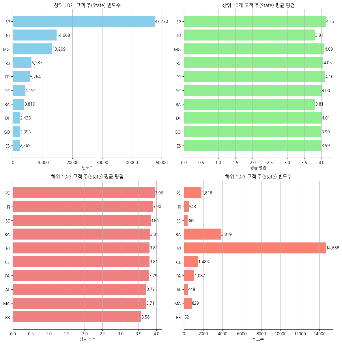
- 고객의 거주 주 별 평균 평점은 3.5 이상으로 나타나며, RJ주는 고객 비중이 높은 주이면서도 평균 평점이 낮은편에 속함
1
2
3
4
5
6
7
8
9
10
11
12
13
14
15
16
low_score_counts = df3_new[df3_new['review_score'].isin([1, 2])].groupby('customer_state')['review_score'].count()

top_low_score_states = low_score_counts.nlargest(10).sort_values(ascending=True)

plt.figure(figsize=(10, 6))
bars = plt.barh(top_low_score_states.index, top_low_score_states.values, color='lightcoral')
plt.title('리뷰점수가 1점 또는 2점이 많은 상위 10개 고객 주(State)')
plt.xlabel('빈도수')
plt.grid(axis='x')

for bar in bars:
    plt.text(bar.get_width(), bar.get_y() + bar.get_height()/2,
             f'{bar.get_width():,.0f}', va='center', ha='left', fontsize=10)

plt.tight_layout()
plt.show()
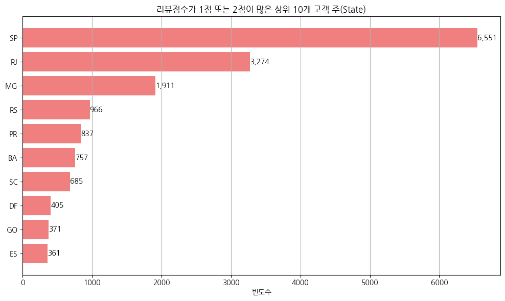
- 거래가 많이되는 곳에 낮은 점수도 많이 분포되고 있음을 알수있다
1
df3_new = df3_new.merge(df4, on='product_id', how='left')
1
2
3
4
5
6
7
8
9
10
11
12
13
14
15
16
17
18
19
20
21
22
23
24
25
26
27
28
29
30
31
32
33
34
35
36
37
38
39
40
41
42
# 1. 1점과 2점인 경우의 수를 계산
low_score_counts = df3_new[df3_new['review_score'].isin([1, 2])].groupby('product_category_name')['review_score'].count()

# 2. 상위 10개 품목 선택
top_low_score_categories = low_score_counts.nlargest(10).sort_values(ascending=True)

# 3. 5점인 경우의 수를 계산
high_score_counts = df3_new[df3_new['review_score'] == 5].groupby('product_category_name')['review_score'].count()

# 4. 상위 10개 품목 선택
top_high_score_categories = high_score_counts.nlargest(10).sort_values(ascending=True)

# 5. subplot 생성
fig, (ax1, ax2) = plt.subplots(1, 2, figsize=(12, 6))

# 6. 첫 번째 차트: 1점 및 2점이 많은 상위 10개 품목
bars1 = ax1.barh(top_low_score_categories.index, top_low_score_categories.values, color='lightcoral')
ax1.set_title('1점 및 2점이 많은 상위 10개 품목')
ax1.set_xlabel('빈도수')
ax1.grid(axis='x')

# 7. 숫자 표기
for bar in bars1:
    ax1.text(bar.get_width(), bar.get_y() + bar.get_height()/2,
             f'{bar.get_width():,.0f}', va='center', ha='left', fontsize=10)

# 8. 두 번째 차트: 5점이 많은 상위 10개 품목
bars2 = ax2.barh(top_high_score_categories.index, top_high_score_categories.values, color='lightgreen')
ax2.set_title('5점이 많은 상위 10개 품목')
ax2.set_xlabel('빈도수')
ax2.grid(axis='x')

for bar in bars2:
    ax2.text(bar.get_width(), bar.get_y() + bar.get_height()/2,
             f'{bar.get_width():,.0f}', va='center', ha='left', fontsize=10)

for ax in [ax1, ax2]:
    ax.spines['top'].set_visible(False)
    ax.spines['right'].set_visible(False)

plt.tight_layout()
plt.show()

- 평점이 높은 카테고리는 낮은 평점도 공존하고있음
현재 주어진 데이터 셋으로 어떤 비즈니스 지표들을 만들 수 있는지 제시하고, 해당 지표들로 AARRR 프레임워크를 구성할 수 있는지 판단하기
Acquisition (획득): 사용자를 획득하는 단계
- 신규 고객 수 :
customer_unique_id활용 신규 고객 수 계산 - 지역별 신규 고객 분포 :
customer_city와customer_state활용 지역별 신규 고객 수 계산
1
2
new_customers = df3_new['customer_unique_id'].nunique()
print("신규 고객 수:", new_customers)
1
신규 고객 수: 95420
1
2
3
4
5
6
7
8
9
10
11
12
13
14
15
16
17
18
19
20
21
22
23
24
25
26
27
28
29
30
31
32
33
34
35
36
37
38
39
40
41
42
43
44
45
46
47
48
49
50
51
52
53
54
55
56
57
58
59
60
61
62
63
64
65
66
67
68
69
70
71
72
73
74
75
76
77
78
# 1. 도시별 신규 고객 수 계산
city_new_customers = df3_new.groupby('customer_city')['customer_unique_id'].nunique()

# 2. 주별 신규 고객 수 계산
state_new_customers = df3_new.groupby('customer_state')['customer_unique_id'].nunique()

# 3. 상위 10개 및 하위 10개 고객 수 선택
top_cities = city_new_customers.nlargest(10).sort_values(ascending=True)
bottom_cities = city_new_customers.nsmallest(10).sort_values(ascending=True)

top_states = state_new_customers.nlargest(10).sort_values(ascending=True)
bottom_states = state_new_customers.nsmallest(10).sort_values(ascending=True)

# 4. subplot 생성
fig, axs = plt.subplots(2, 2, figsize=(14, 12))

# 5. 첫 번째 차트: 상위 10개 도시
bars1 = axs[0, 0].barh(top_cities.index, top_cities.values, color='skyblue')
axs[0, 0].set_title('상위 10개 도시 신규 고객 분포')
axs[0, 0].set_xlabel('신규 고객 수')
axs[0, 0].grid(axis='x')

# 6. 오른쪽과 위쪽 테두리 제거
axs[0, 0].spines['top'].set_visible(False)
axs[0, 0].spines['right'].set_visible(False)

# 7. 숫자 표기
for bar in bars1:
    axs[0, 0].text(bar.get_width(), bar.get_y() + bar.get_height()/2,
                   f'{bar.get_width():,.0f}', va='center', ha='left', fontsize=10)

# 8. 두 번째 차트: 하위 10개 도시
bars2 = axs[0, 1].barh(bottom_cities.index, bottom_cities.values, color='lightcoral')
axs[0, 1].set_title('하위 10개 도시 신규 고객 분포')
axs[0, 1].set_xlabel('신규 고객 수')
axs[0, 1].grid(axis='x')

# 9. 오른쪽과 위쪽 테두리 제거
axs[0, 1].spines['top'].set_visible(False)
axs[0, 1].spines['right'].set_visible(False)

# 10. 숫자 표기
for bar in bars2:
    axs[0, 1].text(bar.get_width(), bar.get_y() + bar.get_height()/2,
                   f'{bar.get_width():,.0f}', va='center', ha='left', fontsize=10)

# 11. 세 번째 차트: 상위 10개 주
bars3 = axs[1, 0].barh(top_states.index, top_states.values, color='lightgreen')
axs[1, 0].set_title('상위 10개 주 신규 고객 분포')
axs[1, 0].set_xlabel('신규 고객 수')
axs[1, 0].grid(axis='x')

# 12. 오른쪽과 위쪽 테두리 제거
axs[1, 0].spines['top'].set_visible(False)
axs[1, 0].spines['right'].set_visible(False)

# 13. 숫자 표기
for bar in bars3:
    axs[1, 0].text(bar.get_width(), bar.get_y() + bar.get_height()/2,
                   f'{bar.get_width():,.0f}', va='center', ha='left', fontsize=10)

# 14. 네 번째 차트: 하위 10개 주
bars4 = axs[1, 1].barh(bottom_states.index, bottom_states.values, color='lightblue')
axs[1, 1].set_title('하위 10개 주 신규 고객 분포')
axs[1, 1].set_xlabel('신규 고객 수')
axs[1, 1].grid(axis='x')

# 15. 오른쪽과 위쪽 테두리 제거
axs[1, 1].spines['top'].set_visible(False)
axs[1, 1].spines['right'].set_visible(False)

# 16. 숫자 표기
for bar in bars4:
    axs[1, 1].text(bar.get_width(), bar.get_y() + bar.get_height()/2,
                   f'{bar.get_width():,.0f}', va='center', ha='left', fontsize=10)

plt.tight_layout()
plt.show()
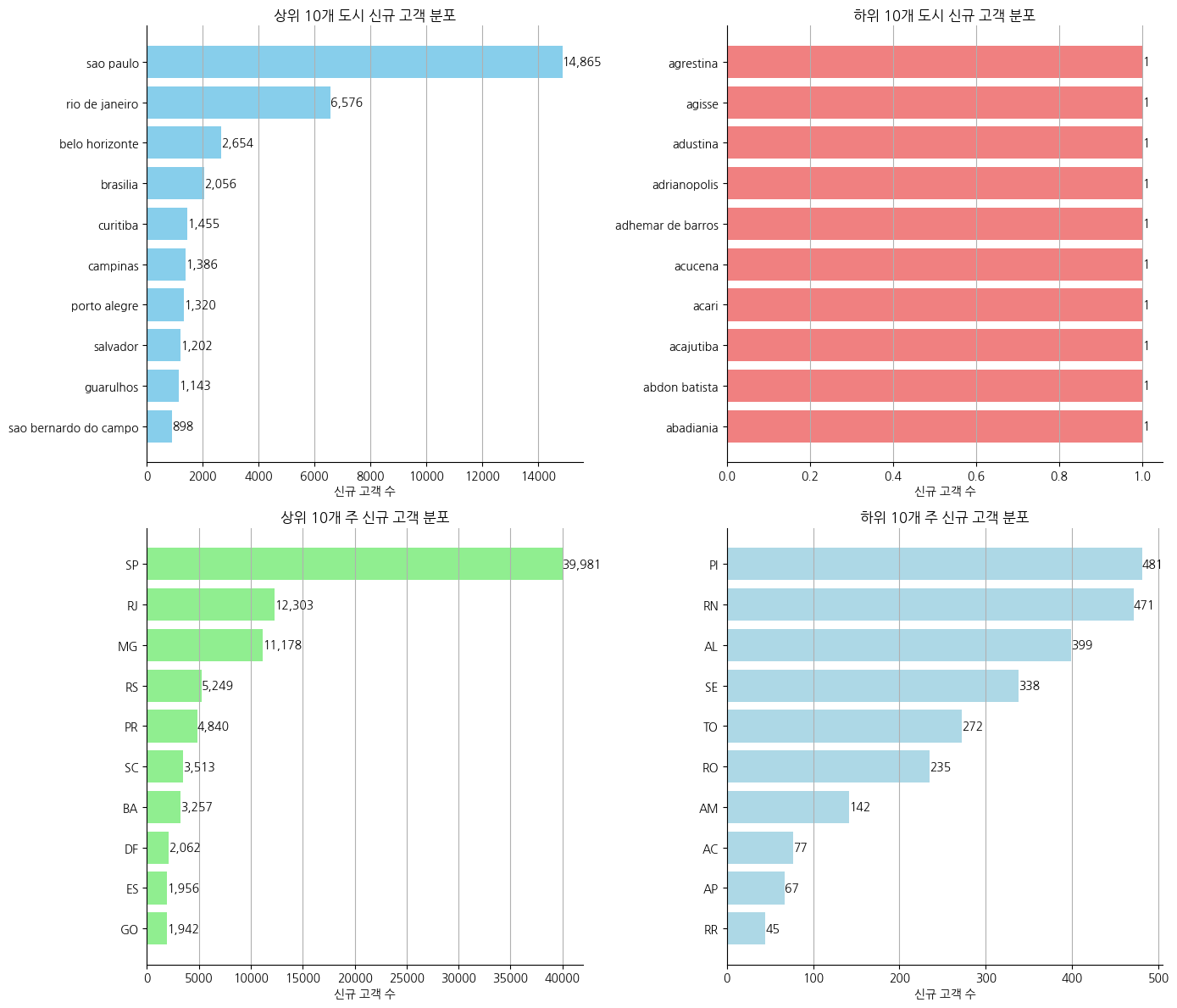
1
state_new_customers.nlargest(3).sum() / new_customers * 100
1
66.50806958708866
1
state_new_customers.nlargest(5).sum() / new_customers * 100
1
77.08132466988053
1
state_new_customers.nlargest(7).sum() / new_customers * 100
1
84.1762733179627
1
2
3
4
5
6
7
8
9
10
11
12
13
14
15
16
17
18
19
20
21
22
23
24
25
26
27
28
29
30
31
32
33
34
35
# 1. customer_state와 seller_state의 빈도수 계산
customer_state_counts = df3_new['customer_state'].value_counts().head(10).sort_values(ascending=True)
seller_state_counts = df3_new['seller_state'].value_counts().head(10).sort_values(ascending=True)

# 2. subplot 생성 (1x2)
fig, (ax1, ax2) = plt.subplots(1, 2, figsize=(14, 6))

# 3. 첫 번째 차트: customer_state 빈도수
bars1 = ax1.barh(customer_state_counts.index, customer_state_counts.values, color='skyblue')
ax1.set_title('상위 10개 고객 주(State) 빈도수')
ax1.set_xlabel('빈도수')
ax1.grid(axis='x')

# 4. 숫자 표기
for bar in bars1:
    ax1.text(bar.get_width(), bar.get_y() + bar.get_height()/2,
             f'{bar.get_width():,.0f}', va='center', ha='left', fontsize=9)

# 5. 두 번째 차트: seller_state 빈도수
bars2 = ax2.barh(seller_state_counts.index, seller_state_counts.values, color='lightgreen')
ax2.set_title('상위 10개 판매자 주(State) 빈도수')
ax2.set_xlabel('빈도수')
ax2.grid(axis='x')

for bar in bars2:
    ax2.text(bar.get_width(), bar.get_y() + bar.get_height()/2,
             f'{bar.get_width():,.0f}', va='center', ha='left', fontsize=9)

ax1.spines['top'].set_visible(False)
ax1.spines['right'].set_visible(False)
ax2.spines['top'].set_visible(False)
ax2.spines['right'].set_visible(False)

plt.tight_layout()
plt.show()
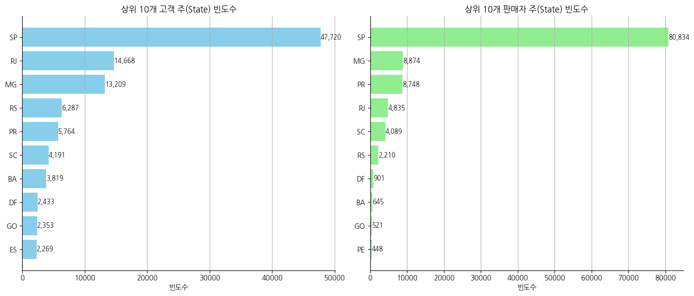
- 전체 고객 중 약 84%가 7개 주(SP, RJ, MG, RS, PR, SC, BA)에서 서비스를 이용하고있다. 판매자도 대부분 7개 주에서 판매를 하고있는것으로 관찰된다.
- 배송비와 타지역 신규유입에 들어가는 시간과 비용을 고려했을때, 전국단위보다는 고객이 모여있는 주를 중심으로 시장을 운영하는것이 효과적으로 보인다
Activation (활성화): 사용자가 제품/서비스를 처음 사용하는 단계
- 첫 구매 완료율 :
order_status가 delivered인 주문 건수를 전체 주문 건수로 나눠서 계산 - 리드 타임 :
order_purchase_timestamp와order_delivered_customer_date컬럼을 이용하여 첫 주문까지의 리드 타임 계산
1
2
3
4
5
6
# 활성화 단계(Activation)
first_purchase_completion_rate = df3_new[df3_new['order_status'] == 'delivered'].shape[0] / df3_new.shape[0]
lead_time = df3_new['delivery_time'].mean()

print("\n첫 구매 완료율:", round(first_purchase_completion_rate * 100, 2))
print("\n리드 타임:", round(lead_time,2))
1
2
3
첫 구매 완료율: 97.82

리드 타임: 12.01
- 데이터 수집기간동안 98% 고객이 구매를 완료하였고, 리드 타임은 평균 12일로 준수함
1
2
3
4
5
6
7
8
9
10
11
12
13
14
15
16
17
18
19
20
21
22
23
24
# 1. 주별 신규 고객 수 계산
state_new_customers = df3_new.groupby('customer_state')['customer_unique_id'].nunique()

# 2. 상위 10개 고객 주 선택
top_states = state_new_customers.nlargest(10).sort_values(ascending=True).index

# 3. 해당 주들의 평균 배송 시간 계산
average_delivery_time = df3_new[df3_new['customer_state'].isin(top_states)].groupby('customer_state')['delivery_time'].mean()

# 4. 평균 배송 시간을 빈도수 기준으로 정렬
average_delivery_time = average_delivery_time.reindex(top_states)

plt.figure(figsize=(10, 6))
bars = plt.barh(average_delivery_time.index, average_delivery_time.values, color='lightblue')
plt.title('상위 10개 고객 주의 평균 배송 시간')
plt.xlabel('평균 배송 시간')
plt.grid(axis='x')

for bar in bars:
    plt.text(bar.get_width(), bar.get_y() + bar.get_height()/2,
             f'{bar.get_width():.2f}', va='center', ha='left', fontsize=10)

plt.tight_layout()
plt.show()
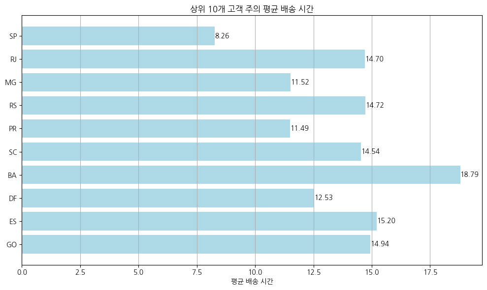
- 국가 특성을 자세히는 모르지만, 상위 10개 고객 주의 리드타임은 대체로 14일 이내로 짧은편이다
1
2
3
4
5
6
7
8
9
10
11
12
13
14
15
16
17
18
19
20
21
22
23
24
25
26
27
# 1. 'review_score'가 1점 또는 2점인 데이터 필터링
filtered_data = df3_new[df3_new['review_score'].isin([1, 2])]

# 2. 주별 신규 고객 수 계산
state_new_customers = filtered_data.groupby('customer_state')['customer_unique_id'].nunique()

# 3. 상위 10개 고객 주 선택
top_states = state_new_customers.nlargest(10).sort_values(ascending=True).index

# 4. 해당 주들의 평균 배송 시간 계산
average_delivery_time = filtered_data[filtered_data['customer_state'].isin(top_states)].groupby('customer_state')['delivery_time'].mean()

# 5. 평균 배송 시간을 빈도수 기준으로 정렬
average_delivery_time = average_delivery_time.reindex(top_states)

plt.figure(figsize=(10, 6))
bars = plt.barh(average_delivery_time.index, average_delivery_time.values, color='lightblue')
plt.title('상위 10개 고객 주의 평균 배송 시간 (리뷰 점수 1점 및 2점)')
plt.xlabel('평균 배송 시간')
plt.grid(axis='x')

for bar in bars:
    plt.text(bar.get_width(), bar.get_y() + bar.get_height()/2,
             f'{bar.get_width():.2f}', va='center', ha='left', fontsize=10)

plt.tight_layout()
plt.show()
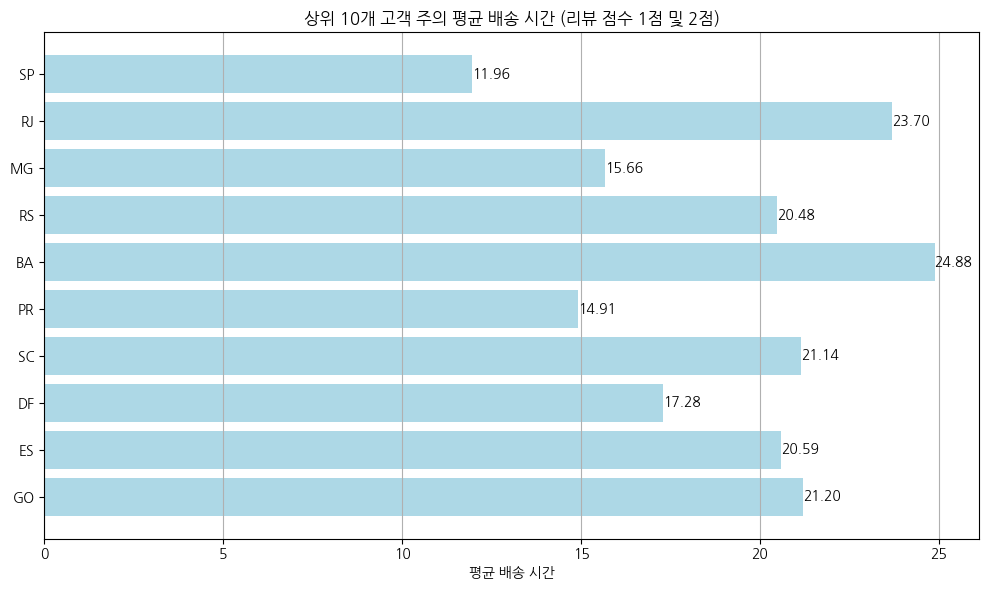
- 평점이 낮은 상품들은 리드 타임이 길어진 경향을 보이고있다. 물리적으로 가능하다면 리드타임을 줄이는 방안을 고민해보고, 구매자와 판매자의 거리상 리드타임이 길어질수밖에 없다면 시스템으로 명확하게 배송기간이 길어질수 있음을 사전에 명시하는 이벤트를 추가하여 고객이 인지하도록 한다. 이를통해 구매를 취소하는 빈도와 평점 등을 종합적으로 고려하여 시스템을 개선해본다
Retention (유지): 사용자가 제품/서비스를 반복적으로 사용하는 단계
- 고객별 주문 횟수 :
customer_unique_id를 이용하여 고객별 주문 횟수 계산 - 코호트별 재구매 분석 :
order_purchase_timestamp를 이용하여 코호트를 구분하고, 각 코호트의 재구매율을 계산 - 이탈 고객 비율 : 특정 기간 동안 구매하지 않은 고객 비율을 계산
1
2
3
customer_order_count = df3_new.groupby('customer_unique_id')['order_id'].nunique()
print("\n고객별 주문 횟수:")
customer_order_count.value_counts()
1
고객별 주문 횟수:
| count | |
|---|---|
| order_id | |
| 1 | 92507 |
| 2 | 2673 |
| 3 | 192 |
| 4 | 29 |
| 5 | 9 |
| 6 | 5 |
| 7 | 3 |
| 9 | 1 |
| 16 | 1 |
1
round(((customer_order_count == 2).sum() / customer_order_count.shape[0])*100,2)
1
2.8
- 대부분 1회성 구매 고객이며, 주문을 2번한 고객은 약 3% 수준으로 관찰됐다. 고객이 재구매를 할수있도록 어떤것들이 문제가있고 개선할 필요가있는지 확인할 필요가 있다
1
2
3
4
5
6
7
8
9
10
11
12
13
14
15
16
17
18
19
20
21
22
df4_new = df3_new.copy()
df4_new['order_purchase_month'] = df4_new['order_purchase_timestamp'].dt.to_period('M')
first_order_month = df4_new.groupby('customer_unique_id')['order_purchase_month'].min()
orders = pd.merge(df4_new, first_order_month.rename('cohort'), on='customer_unique_id')

# 코호트별 재구매율
cohort_repurchase = orders.groupby(['cohort', 'order_purchase_month'])['customer_unique_id'].nunique().reset_index()
cohort_repurchase['period_number'] = (cohort_repurchase['order_purchase_month'] - cohort_repurchase['cohort']).apply(lambda x: x.n)
cohort_pivot = cohort_repurchase.pivot_table(index='cohort', columns='period_number', values='customer_unique_id')
cohort_size = cohort_pivot.iloc[:, 0]
retention_matrix = cohort_pivot.divide(cohort_size, axis=0)

# 시각화: 히트맵 생성
plt.figure(figsize=(12, 8))
sns.heatmap(retention_matrix, annot=True, fmt='.0%', cmap='Blues', cbar_kws={'label': '재구매율'})
plt.title('코호트별 재구매율')
plt.xlabel('기간 번호 (개월)')
plt.ylabel('코호트 (첫 주문 월)')
plt.xticks(rotation=45)
plt.yticks(rotation=0)
plt.tight_layout()
plt.show()
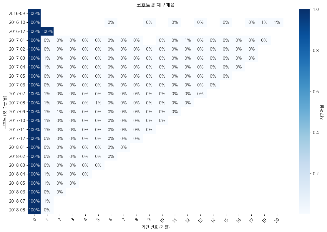
1
2
3
4
5
6
7
8
9
10
11
12
13
# 이탈 고객 비율 계산
churn_rate = 1 - retention_matrix.mean(axis=1)

# 시각화: 이탈 고객 비율 바 차트 생성
plt.figure(figsize=(12, 6))
sns.barplot(x=churn_rate.index.astype(str), y=churn_rate.values, palette='Reds')
plt.title('코호트별 이탈 고객 비율')
plt.xlabel('코호트 (첫 주문 월)')
plt.ylabel('이탈 고객 비율')
plt.xticks(rotation=45)
plt.ylim(0, 1)  # 비율이 0%에서 100%까지이므로 y축 범위를 설정
plt.tight_layout()
plt.show()
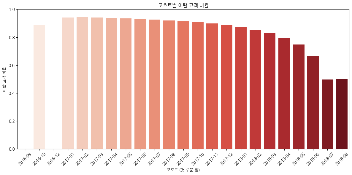
1
churn_rate
| 0 | |
|---|---|
| cohort | |
| 2016-09 | 0.000000 |
| 2016-10 | 0.885246 |
| 2016-12 | 0.000000 |
| 2017-01 | 0.941866 |
| 2017-02 | 0.942750 |
| 2017-03 | 0.942175 |
| 2017-04 | 0.939114 |
| 2017-05 | 0.934744 |
| 2017-06 | 0.930679 |
| 2017-07 | 0.926174 |
| 2017-08 | 0.920352 |
| 2017-09 | 0.913794 |
| 2017-10 | 0.906598 |
| 2017-11 | 0.898005 |
| 2017-12 | 0.886990 |
| 2018-01 | 0.872691 |
| 2018-02 | 0.854629 |
| 2018-03 | 0.831174 |
| 2018-04 | 0.797466 |
| 2018-05 | 0.747464 |
| 2018-06 | 0.664364 |
| 2018-07 | 0.497440 |
| 2018-08 | 0.499920 |
- 월별 코호트 분석을 수행해도 앞서 고객별 주문 횟수를 확인한 결과와 동일하게 대부분의 고객(90% 이상)이 1회 구매후 이탈하고있다. (2018년도 데이터는 거래가 작아서 이탈율이 전월대비 낮아보인다)
- 앞서 EDA진행시 제품 평점은 5점 비율이 높았으며, 평균 평점도 제일 낮은지역도 3.5이상으로 나타났다. 그럼에도 이탈률이 높다는 것은 마케팅 전략이나 서비스 품질이 문제가 있다고 판단할 수 있다.
- 고객 유지 전략을 강화하기위해 고객 경험을 개선할 필요가 있다. 예를들어, 고객의 피드백을 수용하는 시스템을 만들거나 프로모션이나 서비스 개선을 검토해볼 수 있다
Revenue (수익): 사용자가 제품/서비스를 통해 수익을 창출하는 단계
- 총 매출 :
price컬럼의 합 계산 - 평균 주문 금액 :
price컬럼과order_purchase_timestamp이용하여 평균 주문 금액 계산 - 카테고리별 매출 분석 :
price와product_category_name을 이용하여 카테고리별 매출 계산
1
print("\n총 매출:", df3_new['price'].sum())
1
총 매출: 13651923.47
1
2
3
4
5
6
7
8
9
10
11
12
13
14
15
16
17
18
19
20
21
22
23
24
25
26
27
28
29
30
31
32
33
34
35
36
37
38
39
40
41
42
43
44
45
46
47
48
# 연도와 월별로 그룹화하여 주문 수 계산
monthly_orders = df2.groupby(df2['order_purchase_timestamp'].dt.to_period('M')).size()

# 1. 'shipping_limit_date'를 datetime 형식으로 변환
df3['shipping_limit_date'] = pd.to_datetime(df3['shipping_limit_date'])

# 2. 월별 매출액 집계
monthly_sales = df3.resample('M', on='shipping_limit_date')['price'].sum()

# 3. 2018년 8월까지의 데이터만 필터링
monthly_sales = monthly_sales[monthly_sales.index <= '2018-08-31']

# 4. subplot 생성
fig, (ax1, ax2) = plt.subplots(2, 1, figsize=(10, 12))

# 첫 번째 차트: 월별 주문 수
bars = ax1.bar(monthly_orders.index.astype(str), monthly_orders.values, color='skyblue')

# 주문 수 표시
for bar in bars:
    yval = bar.get_height()
    ax1.text(bar.get_x() + bar.get_width()/2, yval, str(yval), ha='center', va='bottom')

ax1.set_title('월별 주문 수')
ax1.set_xlabel('연도-월')
ax1.set_ylabel('주문 수')
ax1.set_xticks(range(len(monthly_orders.index)))  # x축 위치 설정
ax1.set_xticklabels(monthly_orders.index.astype(str), rotation=45)  # 레이블과 회전 설정
ax1.grid(axis='y')

# 두 번째 차트: 월별 매출액 추이
ax2.plot(monthly_sales.index, monthly_sales.values, marker='o')

# 매출액 숫자 표기
for x, y in zip(monthly_sales.index, monthly_sales.values):
    ax2.text(x, y, f'{y:,.0f}', fontsize=9, ha='center', va='bottom')

# x축을 3개월 단위로 설정
ax2.set_xticks(monthly_sales.index[::3])
ax2.set_title('월별 매출액 추이')
ax2.set_xlabel('월')
ax2.set_ylabel('매출액')
ax2.set_xlim(pd.Timestamp('2016-09-01'), pd.Timestamp('2018-08-31'))  # x축 범위 설정
ax2.grid()

# 레이아웃 조정 및 그래프 표시
plt.tight_layout()
plt.show()
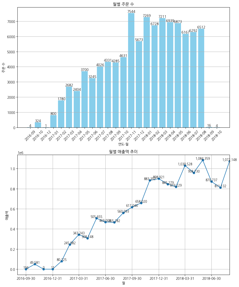
- 제품 판매수와 매출은 상승곡선을 그리고있다. 리텐션을 개선한다면 수익을 극대화 할 수 있다. 획득부분에서 얻은 고객이 거주하는 상위 3개 주를 우선적으로 마케팅 전략을 세우고, 상위 7개 주까지 확대방안을 검토해본다.
1
2
3
4
5
6
7
8
9
10
11
12
13
14
15
# 코호트 분석을 위한 평균 주문 금액 계산
cohort_order_value = orders.groupby(['cohort', 'order_purchase_month'])['price'].mean().reset_index()
cohort_order_value['period_number'] = (cohort_order_value['order_purchase_month'] - cohort_order_value['cohort']).apply(lambda x: x.n)
cohort_order_value_pivot = cohort_order_value.pivot_table(index='cohort', columns='period_number', values='price')

plt.figure(figsize=(12, 8))
sns.heatmap(cohort_order_value_pivot, annot=True, fmt='.0f', cmap='YlGnBu', cbar_kws={'label': '평균 주문 금액'})
plt.title('코호트별 평균 주문 금액')
plt.xlabel('기간 번호 (개월)')
plt.ylabel('코호트 (첫 주문 월)')
plt.xticks(rotation=45)
plt.yticks(rotation=0)
plt.tight_layout()
plt.show()
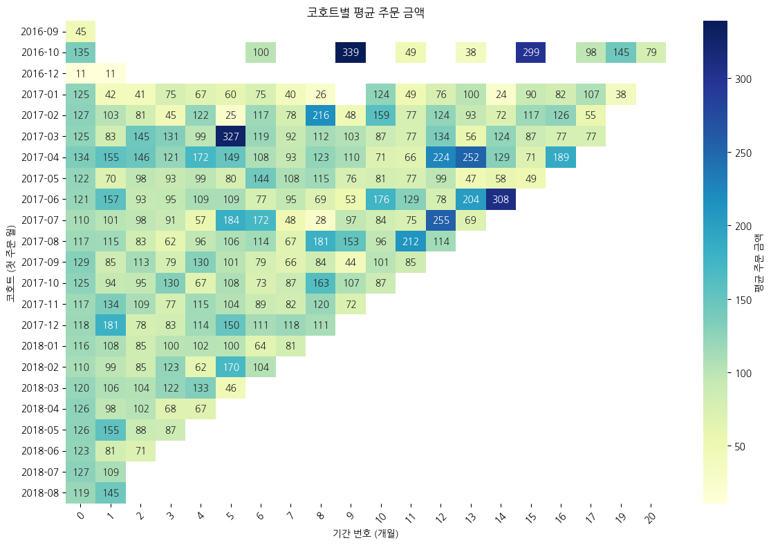
- 대부분의 코호트는 평균주문금액이 초기의 높게 형성됐으며, 시간이 지남에 따라 감소하는 경향을 보이고있다. 다만, 앞서 살펴본 재구매율이 3%수준이기 때문에 근본적으로 고객이 재구매할 수 있는 환경을 조성해야한다
1
2
3
4
5
6
7
8
9
10
11
12
13
14
15
16
17
18
19
20
21
22
23
24
25
26
27
28
29
30
31
32
33
34
35
36
37
38
39
40
41
42
43
44
45
46
47
48
49
50
51
52
53
54
55
56
57
58
# 1. 'product_category_name'에 대한 빈도수 계산
category_counts = merged_df_product['product_category_name'].value_counts()
category_revenue = merged_df_product.groupby('product_category_name')['price'].sum()

# 2. 전체 매출액 및 전체 빈도수 계산
total_revenue = category_revenue.sum()
total_count = category_counts.sum()

# 3. 첫 번째 줄을 위한 상위 10개 카테고리 선택 및 정렬
top_categories_counts = category_counts.head(10).sort_values(ascending=True)
top_categories_revenue = category_revenue[top_categories_counts.index]

# 4. 상위 10개 카테고리의 매출 비중 및 빈도 비중 계산
top_revenue_percentage = (top_categories_revenue / total_revenue) * 100
top_count_percentage = (top_categories_counts / total_count) * 100

# 5. subplot 생성 (2x2)
fig, ((ax1, ax2), (ax3, ax4)) = plt.subplots(2, 2, figsize=(14, 10))

# 6. 차트 생성 함수
def create_bar_chart(ax, x_data, y_data, title, xlabel, color):
    bars = ax.barh(x_data, y_data, color=color)
    ax.set_title(title)
    ax.set_xlabel(xlabel)
    ax.grid(axis='x')
    for bar in bars:
        ax.text(bar.get_width(), bar.get_y() + bar.get_height()/2,
                f'{bar.get_width():,.1f}%', va='center', ha='left', fontsize=9)

# 7. 첫 번째 차트: 'product_category_name' 빈도수 비중 (상위 10개)
create_bar_chart(ax1, top_categories_counts.index, top_count_percentage,
                 '상품 카테고리별 빈도수 비중 (%) (상위 10개)', '빈도수 비중 (%)', 'skyblue')

# 8. 두 번째 차트: 상위 10개 카테고리의 매출 비중
create_bar_chart(ax2, top_categories_counts.index, top_revenue_percentage,
                 '상품 카테고리별 매출 비중 (%) (상위 10개)', '매출 비중 (%)', 'lightgreen')

# 9. 세 번째 차트: 전체 매출액 상위 10개의 상품 카테고리 비중
top_revenue_categories = category_revenue.nlargest(10).sort_values(ascending=True)
top_revenue_categories_percentage = (top_revenue_categories / total_revenue) * 100
create_bar_chart(ax3, top_revenue_categories.index, top_revenue_categories_percentage,
                 '총 매출액 상위 10개 상품 카테고리 비중 (%)', '매출 비중 (%)', 'orange')

# 10. 네 번째 차트: 빈도수 (상위 10개 카테고리, 비중)
top_revenue_categories_counts = category_counts[top_revenue_categories.index]
top_revenue_categories_counts_percentage = (top_revenue_categories_counts / total_count) * 100
create_bar_chart(ax4, top_revenue_categories.index, top_revenue_categories_counts_percentage,
                 '상품 카테고리별 빈도수 비중 (%) (상위 10개)', '빈도수 비중 (%)', 'skyblue')

ax2.yaxis.set_visible(False)
ax4.yaxis.set_visible(False)

for ax in [ax1, ax2, ax3, ax4]:
    ax.spines['top'].set_visible(False)
    ax.spines['right'].set_visible(False)

plt.tight_layout()
plt.show()
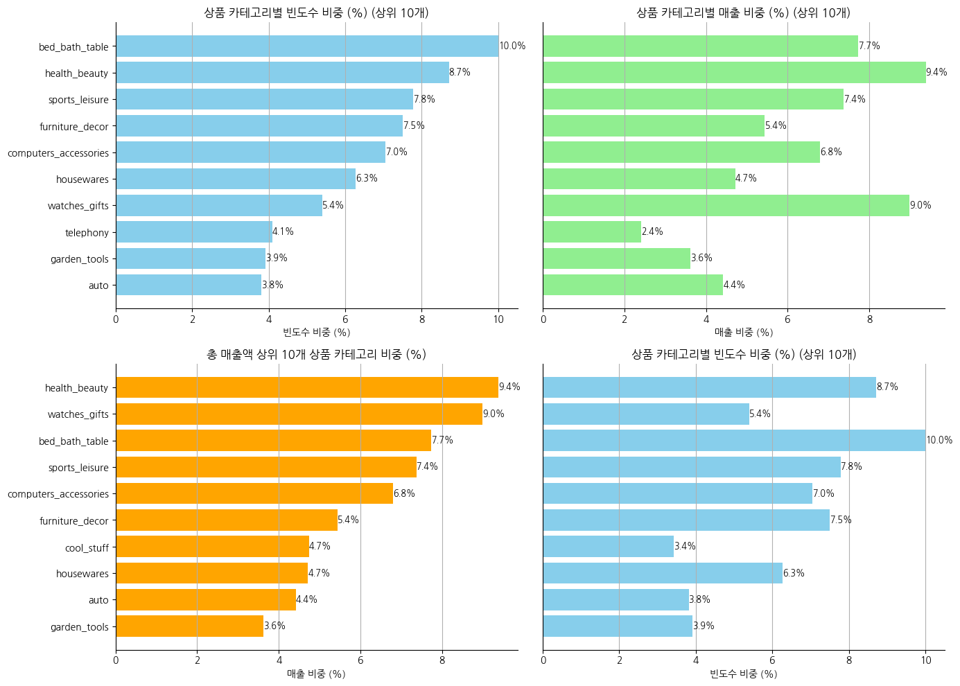
- 판매량과 매출액이 반드시 비례하는것은 아닌것으로 관찰됨
- 특정 카테고리 매출비중이 높지않고 고르게 매출이 발생하고있으며, 건강과 미용 상품과 선물용 시계 상품이 각각 전체매출에 약 9% 비중을 차지하는 상위품목으로 관찰됨
1
2
3
4
5
6
7
8
9
10
11
12
13
14
15
16
17
18
19
20
21
22
23
24
25
26
total_sales_by_state = df3_new.groupby('customer_state')['price'].sum().reset_index()

# 전체 매출액 계산
total_sales = total_sales_by_state['price'].sum()

# 퍼센트 계산
total_sales_by_state['percentage'] = (total_sales_by_state['price'] / total_sales) * 100

# 매출액 기준으로 상위 10개 주 선택
top_10_states = total_sales_by_state.nlargest(10, 'price')

# 시각화: 상위 10개 주의 총 매출액 차트
plt.figure(figsize=(10, 6))
bars = sns.barplot(y='customer_state', x='price', data=top_10_states.sort_values(by='price', ascending=False), palette='Blues')
plt.title('고객 주별 총 매출액 상위 10개 (퍼센트 포함)')
plt.xlabel('총 매출액')
plt.ylabel('고객 주')

# 퍼센트 표시
for index, bar in enumerate(bars.patches):
    plt.text(bar.get_x() + bar.get_width() + 10000, bar.get_y() + bar.get_height() / 2,
             f'{top_10_states["percentage"].iloc[index]:.1f}%', color='black', va='center')

plt.tight_layout()
plt.show()
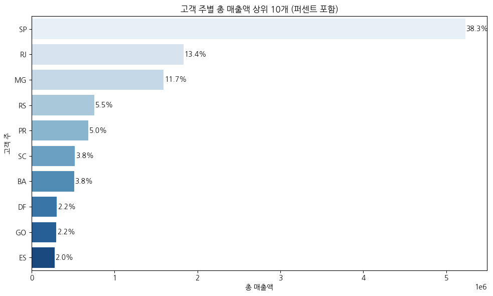
- 매출 비중은 SP에서 약 40%로 대부분의 매출이 발생하고있으며, 상위 5개 주를 포함하면 74%에 해당되고있다.
1
2
3
4
5
6
7
8
9
10
11
12
13
14
15
16
17
18
19
20
21
22
23
24
25
26
27
28
29
30
31
32
33
34
35
36
37
38
39
40
41
42
43
44
45
46
47
48
49
50
top_states = df3_new['customer_state'].value_counts().nlargest(5).index

# 상위 5개 주에서의 총 매출액 계산
top_states_data = df3_new[df3_new['customer_state'].isin(top_states)]
total_sales_by_category = top_states_data.groupby('product_category_name')['price'].sum().reset_index()

# 매출액 기준으로 상위 10개 상품 카테고리 선택
top_10_categories = total_sales_by_category.nlargest(10, 'price')

# 전체 매출액 계산
total_sales = top_states_data['price'].sum()

# 퍼센트 계산
top_10_categories['percentage'] = (top_10_categories['price'] / total_sales) * 100

# 상품 카테고리 상위 10개 계산
category_counts = top_states_data['product_category_name'].value_counts().nlargest(10).reset_index()
category_counts.columns = ['product_category_name', 'count']

# 시각화: 서브플롯 생성
fig, axes = plt.subplots(1, 2, figsize=(15, 6))

# 첫 번째 차트: 상위 10개 상품 카테고리 총 매출액
bars1 = sns.barplot(y='product_category_name', x='price', data=top_10_categories, palette='Blues', ax=axes[0])
axes[0].set_title('고객 상위 5개 주(state)의 상위 10개 상품 카테고리 총 매출액')
axes[0].set_xlabel('총 매출액')
axes[0].set_ylabel('상품 카테고리')

# 퍼센트 표시
for index, bar in enumerate(bars1.patches):
    axes[0].text(bar.get_x() + bar.get_width() + 10000, bar.get_y() + bar.get_height() / 2,
                  f'{top_10_categories["percentage"].iloc[index]:.1f}%', color='black', va='center')

# 두 번째 차트: 상품 카테고리 상위 10개
bars2 = sns.barplot(y='product_category_name', x='count', data=category_counts, palette='Greens', ax=axes[1])
axes[1].set_title('고객 상위 5개 주(state)의 상품 카테고리 상위 10개')
axes[1].set_xlabel('주문 수')
axes[1].set_ylabel('상품 카테고리')

# 퍼센트 표시
total_count = category_counts['count'].sum()
for index, row in category_counts.iterrows():
    axes[1].text(row['count'] + 0.5, index, f'{(row["count"] / total_count) * 100:.1f}%', color='black', va='center')

for ax in axes:
    ax.spines['top'].set_visible(False)
    ax.spines['right'].set_visible(False)

plt.tight_layout()
plt.show()
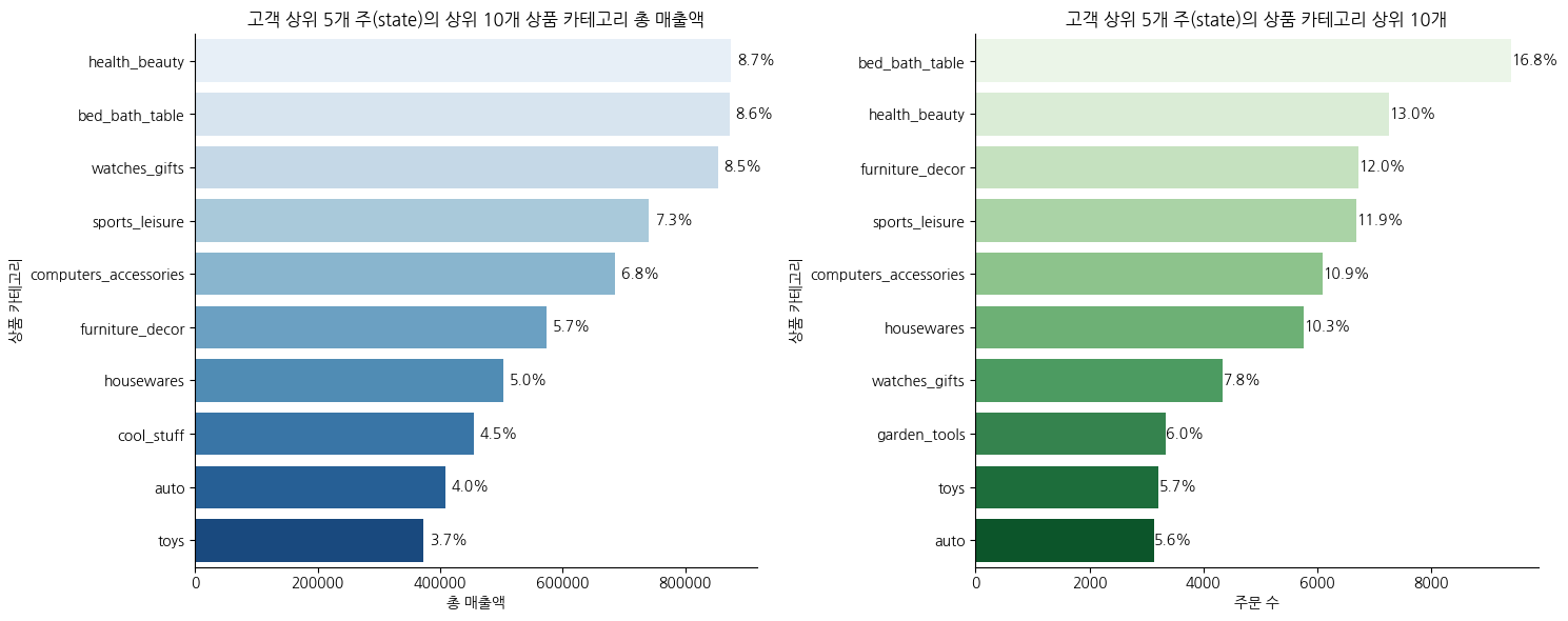
- olist 이용 고객 77%가 속한 상위 5개 주(state)기준 상위 10개 상품 카테고리가 약 63% 매출 비중을 차지한다. 즉, 전체 매출 74% 중 63%의 매출이 상위 10개 상품 카테고리에서 발생하고 있다
- 수익을 우선적으로 극대화하기 위해 상위 5개 주에서 매출비중이 높은 상품을 확장시키는 방안을 검토해본다.
- 다양한 상품은 전지역에 파는 방향보다는 잘팔리는 상품을 구매자와 판매자가 밀집된 지역에 우선적으로 마케팅 전략을 세우는 방향을 도입해볼 필요가 있다
Referral (추천): 사용자가 제품/서비스를 다른 사람에게 추천하는 단계
- 제품별/카테고리별 평점 비교 :
product_id,product_category_name과review_score컬럼을 이용하여 제품별 평점 비교 - 순 추천지수 : 리뷰 점수를 추천그룹(5점)과 비추천그룹(1점,2점)의 비율을 계산
1
2
3
product_ratings = round(df3_new.groupby('product_category_name')['review_score'].mean(),2).sort_values(ascending=False).reset_index()
print("\n카테고리별 평점 비교:")
product_ratings
1
카테고리별 평점 비교:
| product_category_name | review_score | |
|---|---|---|
| 0 | cds_dvds_musicals | 4.64 |
| 1 | fashion_childrens_clothes | 4.50 |
| 2 | books_general_interest | 4.45 |
| 3 | costruction_tools_tools | 4.44 |
| 4 | flowers | 4.42 |
| ... | ... | ... |
| 68 | office_furniture | 3.49 |
| 69 | pc_gamer | 3.33 |
| 70 | portateis_cozinha_e_preparadores_de_alimentos | 3.27 |
| 71 | diapers_and_hygiene | 3.26 |
| 72 | security_and_services | 2.50 |
73 rows × 2 columns
1
product_ratings.nlargest(10, 'review_score')
| product_category_name | review_score | |
|---|---|---|
| 11 | cds_dvds_musicals | 4.64 |
| 29 | fashion_childrens_clothes | 4.50 |
| 8 | books_general_interest | 4.45 |
| 22 | costruction_tools_tools | 4.44 |
| 35 | flowers | 4.42 |
| 9 | books_imported | 4.40 |
| 10 | books_technical | 4.37 |
| 37 | food_drink | 4.32 |
| 53 | luggage_accessories | 4.32 |
| 66 | small_appliances_home_oven_and_coffee | 4.30 |
1
product_ratings.nsmallest(10, 'review_score')
| product_category_name | review_score | |
|---|---|---|
| 63 | security_and_services | 2.50 |
| 23 | diapers_and_hygiene | 3.26 |
| 62 | portateis_cozinha_e_preparadores_de_alimentos | 3.27 |
| 59 | pc_gamer | 3.33 |
| 57 | office_furniture | 3.49 |
| 46 | home_comfort_2 | 3.63 |
| 30 | fashion_male_clothing | 3.64 |
| 34 | fixed_telephony | 3.68 |
| 58 | party_supplies | 3.77 |
| 27 | fashio_female_clothing | 3.78 |
1
2
3
4
5
6
7
8
9
10
11
12
13
14
15
16
17
18
19
20
21
22
23
24
25
product_ratings = round(df3_new.groupby('product_category_name')['review_score'].mean(), 2).reset_index()

# 상위 10개와 하위 10개 상품 카테고리 선택
top_10_categories = product_ratings.nlargest(10, 'review_score')
bottom_10_categories = product_ratings.nsmallest(10, 'review_score')

# 상위 10개와 하위 10개를 하나의 데이터프레임으로 결합
top_10_categories['category_type'] = '상위'
bottom_10_categories['category_type'] = '하위'
combined_categories = pd.concat([top_10_categories, bottom_10_categories])

# 시각화: 평균 평점 차트
plt.figure(figsize=(10, 6))
bars = sns.barplot(y='product_category_name', x='review_score', data=combined_categories.sort_values(by='review_score', ascending=False), palette='coolwarm', hue='category_type')
plt.title('상품 카테고리 평균 평점 (상위 10개 및 하위 10개)')
plt.xlabel('평균 평점')
plt.ylabel('상품 카테고리')

# 평균 평점 표시
for index, bar in enumerate(bars.patches):
    plt.text(bar.get_x() + bar.get_width() + 0.01, bar.get_y() + bar.get_height() / 2,
             f'{bar.get_width():.2f}', color='black', va='center')

plt.tight_layout()
plt.show()
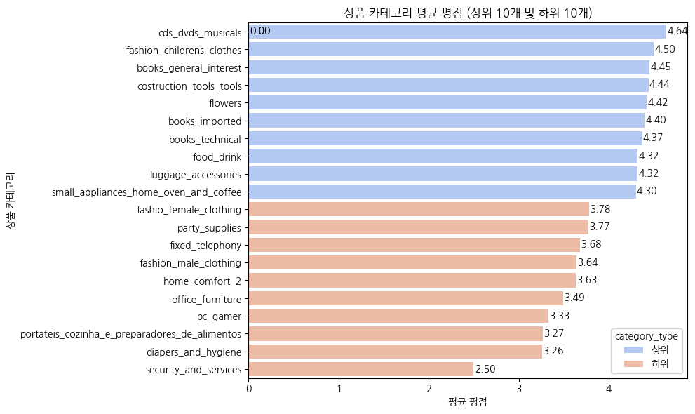
1
2
3
4
5
6
7
8
9
10
11
12
13
14
15
16
17
18
19
20
21
22
23
24
25
26
27
28
29
30
31
32
33
34
35
36
37
38
39
40
41
42
# 1. 1점과 2점인 경우의 수를 계산
low_score_counts = df3_new[df3_new['review_score'].isin([1, 2])].groupby('product_category_name')['review_score'].count()

# 2. 상위 10개 품목 선택
top_low_score_categories = low_score_counts.nlargest(10).sort_values(ascending=True)

# 3. 5점인 경우의 수를 계산
high_score_counts = df3_new[df3_new['review_score'] == 5].groupby('product_category_name')['review_score'].count()

# 4. 상위 10개 품목 선택
top_high_score_categories = high_score_counts.nlargest(10).sort_values(ascending=True)

# 5. subplot 생성
fig, (ax1, ax2) = plt.subplots(1, 2, figsize=(12, 6))

# 6. 첫 번째 차트: 1점 및 2점이 많은 상위 10개 품목
bars1 = ax1.barh(top_low_score_categories.index, top_low_score_categories.values, color='lightcoral')
ax1.set_title('1점 및 2점이 많은 상위 10개 품목')
ax1.set_xlabel('빈도수')
ax1.grid(axis='x')

# 7. 숫자 표기
for bar in bars1:
    ax1.text(bar.get_width(), bar.get_y() + bar.get_height()/2,
             f'{bar.get_width():,.0f}', va='center', ha='left', fontsize=10)

# 8. 두 번째 차트: 5점이 많은 상위 10개 품목
bars2 = ax2.barh(top_high_score_categories.index, top_high_score_categories.values, color='lightgreen')
ax2.set_title('5점이 많은 상위 10개 품목')
ax2.set_xlabel('빈도수')
ax2.grid(axis='x')

for bar in bars2:
    ax2.text(bar.get_width(), bar.get_y() + bar.get_height()/2,
             f'{bar.get_width():,.0f}', va='center', ha='left', fontsize=10)

for ax in [ax1, ax2]:
    ax.spines['top'].set_visible(False)
    ax.spines['right'].set_visible(False)

plt.tight_layout()
plt.show()
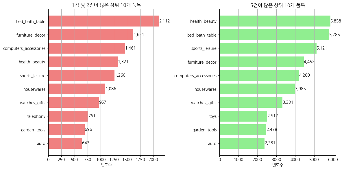
- 잘팔리는 상품들은 하위 평점은 아니지만 낮은평점과 높은평점이 공존하고있다
- aarrr 관점에서 우리는 고객이 밀집한 주(state)에서 잘팔리는 상품들을 확대하기로 설정했다.
- 따라서 잘팔리는 상품들의 평점이 1점이나 2점을 받은 낮은 사례들의 리뷰를 확인해서 고객의 피드백을 반영하도록 노력한다
- 추가적으로 리드타임이 길어지면 평점이 낮아지는 경향을 활성화 단계에서 발견했다. 이부분도 리드타임을 개선할 수 있는 방안이나 고객이 인지할수있는 방안을 강구해본다
1
2
3
4
5
6
7
8
9
10
11
12
13
14
15
16
17
18
19
20
21
22
23
24
25
26
27
df3_new['review_answer_timestamp'] = pd.to_datetime(df3_new['review_answer_timestamp'])

# 추천 및 비추천 그룹 분류
df3_new['group'] = df3_new['review_score'].apply(lambda x: '추천' if x == 5 else ('비추천' if x in [1, 2] else '중립'))

# 월별 집계
df3_new['month'] = df3_new['review_answer_timestamp'].dt.to_period('M')
monthly_counts = df3_new.groupby(['month', 'group']).size().unstack(fill_value=0)

# NPS 계산
monthly_counts['NPS'] = (monthly_counts['추천'] - monthly_counts['비추천']) / (monthly_counts['추천'] + monthly_counts['비추천']) * 100

# 시각화
plt.figure(figsize=(12, 6))
sns.lineplot(data=monthly_counts, x=monthly_counts.index.astype(str), y='NPS', marker='o')
plt.title('월별 NPS (추천 비율 - 비추천 비율)')
plt.xlabel('월')
plt.ylabel('NPS (%)')
plt.xticks(rotation=45)
plt.axhline(0, color='red', linestyle='--', linewidth=1)

# NPS 값 표시
for i, nps_value in enumerate(monthly_counts['NPS']):
    plt.text(i, nps_value, f'{nps_value:.1f}', color='black', ha='center', va='bottom')

plt.tight_layout()
plt.show()
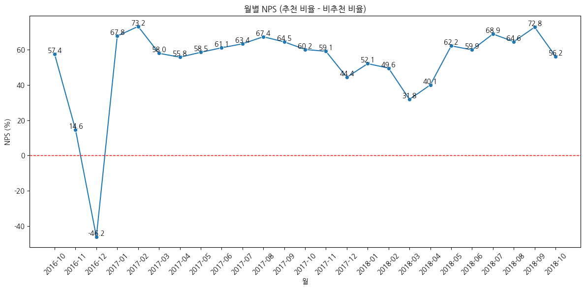
- 월별 순 추천지수(NPS)는 대부분 40점 이상으로 굉장히 높게 나타났는데, 실제 재구매율은 3%로 굉장히 낮은 수치를 보이고있다. 리뷰를 5점을 주는것이 과장된 부분이 없는지(리뷰이벤트나 평점을 조작하지 않았는지 등) 감안할 필요가 있다.
- 재구매율을 감안했을때 리뷰점수가 낮은 1점과 2점을 진실된 리뷰로 해석할 수도 있다. 따라서 평점이 낮은 부분을 적극적으로 확인하고, 추가적으로 리뷰 외에도 설문조사 등으로 고객의 의견을 받을 수 있도록 다양한 채널을 만들어 확인할 필요가 있다.
This post is licensed under CC BY 4.0 by the author.