파이썬 데이터분석 클러스터와 차원축소
- 고객의 정기예금 가입 여부 예측을 위한 은행 마케팅 분류 모델 구축
- 자전거 대여 수요 예측을 위한 머신러닝 모델 구축
- 파이썬 데이터분석 - A/B test 분석
- 파이썬 데이터분석 - aarrr 분석 실습
- 파이썬 데이터분석 - 장바구니 분석(연관분석)2 - FP-Growth, 순차패턴마이닝
- 파이썬 데이터분석 - 장바구니 분석(연관분석) 실습
- 파이썬 데이터분석 - 장바구니 분석(연관분석)
- 파이썬 데이터분석 데이터시각화 실습
- 파이썬 데이터분석 데이터시각화2
- 파이썬 데이터분석 데이터시각화1
- 파이썬 데이터분석 클러스터와 차원축소 실습
- 파이썬 데이터분석 클러스터와 차원축소2
- 파이썬 데이터분석 라이브러리
클러스터링 연습
클러스터 예제 1
1
2
3
4
import pandas as pd

user_activity = pd.read_csv('/content/drive/MyDrive/app_users.csv', encoding='utf-8-sig', index_col=[0])
user_activity.head()
| visit_per_month | use_time | |
|---|---|---|
| 0 | 14 | 22.8 |
| 1 | 32 | 13.6 |
| 2 | 8 | 3.1 |
| 3 | 13 | 5.7 |
| 4 | 19 | 20.8 |
1
2
3
4
5
6
7
8
9
import seaborn as sns
sns.set(style='darkgrid',
rc={'figure.figsize':(16,9)})
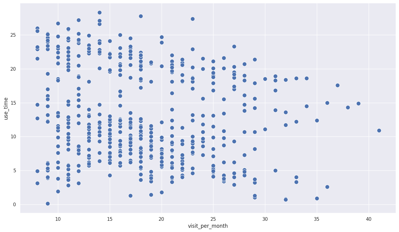
# 산점도 시각화
sns.scatterplot(x='visit_per_month', y='use_time', data=user_activity,
s=100, palette='bright')
# 데이터가 넓게 분포해있어 다른접근필요
1
2
3
4
5
6
7
8
<ipython-input-22-4eeb1d927849>:6: UserWarning: Ignoring `palette` because no `hue` variable has been assigned.
  sns.scatterplot(x='visit_per_month', y='use_time', data=user_activity,


<Axes: xlabel='visit_per_month', ylabel='use_time'>
1
2
3
4
5
6
7
8
9
from sklearn.cluster import KMeans
model = KMeans(n_clusters=3, random_state=123)
model.fit(user_activity)

# 클러스터 구분
user_activity['label'] = model.predict(user_activity)

# 클러스터별 속한 유저 수
user_activity.groupby('label').count()
1
2
/usr/local/lib/python3.10/dist-packages/sklearn/cluster/_kmeans.py:1416: FutureWarning: The default value of `n_init` will change from 10 to 'auto' in 1.4. Set the value of `n_init` explicitly to suppress the warning
  super()._check_params_vs_input(X, default_n_init=10)
| visit_per_month | use_time | |
|---|---|---|
| label | ||
| 0 | 228 | 228 |
| 1 | 126 | 126 |
| 2 | 146 | 146 |
1
2
3
4
5
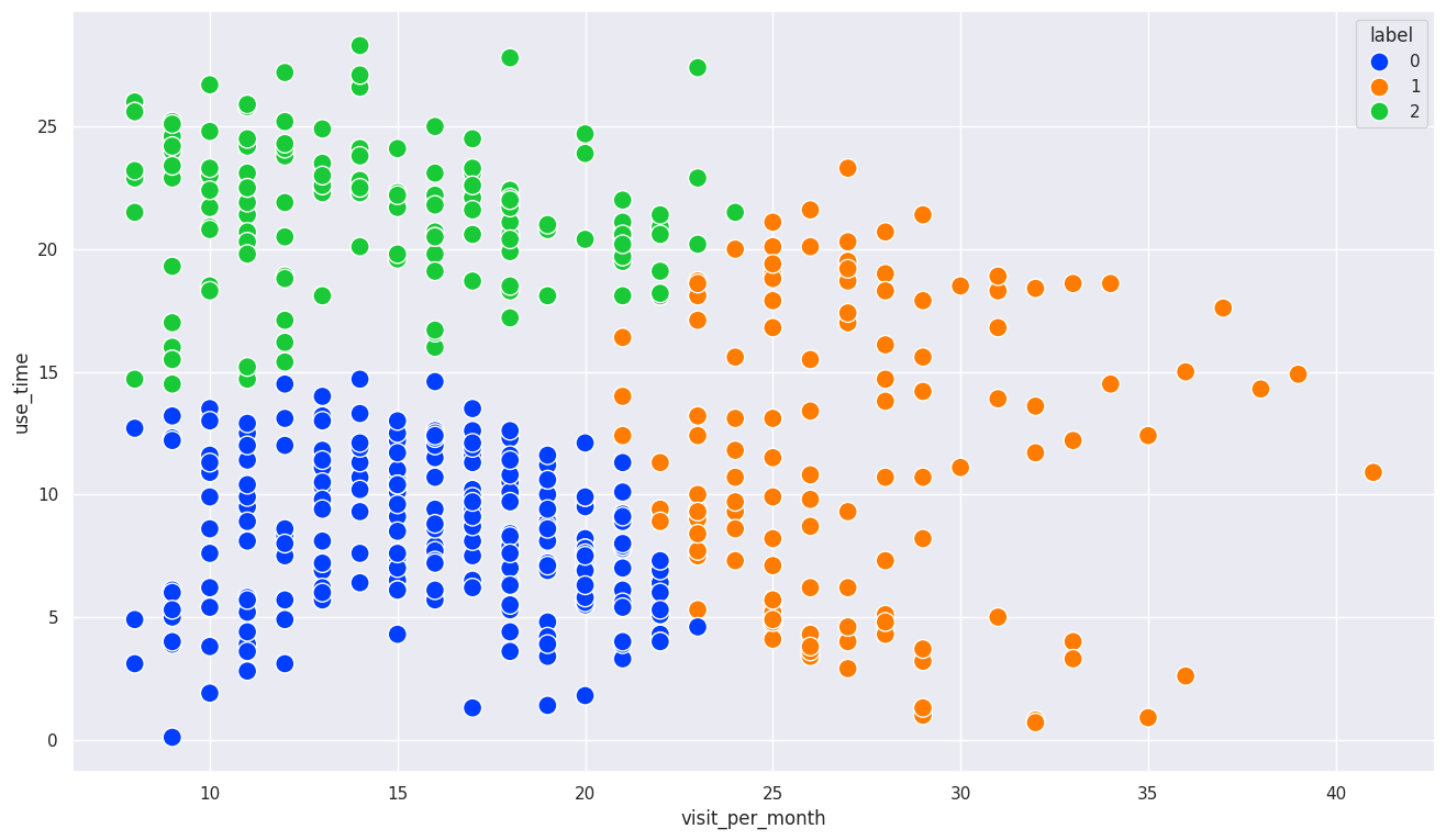
# 클러스터로 구분된 데이터들을 산점도로 색깔로 표시
sns.scatterplot(x='visit_per_month', y='use_time',
data=user_activity, hue=user_activity['label'],
s = 150, palette='bright')
# hue : 데이터 포인트의 색상을 선택한 변수별로 다르게 해주는 옵션
1
<Axes: xlabel='visit_per_month', ylabel='use_time'>
1
user_activity.columns
1
Index(['visit_per_month', 'use_time', 'label'], dtype='object')
1
2
3
4
5
6
7
8
9
10
11
12
13
14
15
16
17
18
19
# 클러스터별 통계 계산
user_activity['label'] = user_activity['label'].astype(str).replace({'0': '실속형', '1': '꾸준형', '2': '탐구형'})

summary = user_activity.groupby('label').agg(
    user = ('use_time', 'count'),
    visit_month = ('visit_per_month', 'mean'),
    time_month = ('use_time', 'mean')
)
summary['visit_month'] = summary['visit_month'].round(1)
summary['time_month'] = summary['time_month'].round(1)

summary.rename(columns={'user':'포함된 유저 수','visit_month':'월 방문 횟수(평균)','time_month':'월 사용 시간(평균)'}, inplace=True)


summary

# 꾸준형 : 보상이나 기록 등 특정목적을 가지고 방문하는 유형, 출석이벤트나 개인기록에 관심이나 신경을 쓰는 사람, 방문목적이 자신으로 귀결되고 방문한곳의 관심도는 낮을수있음
# 실속형 : 방문했을때 관심있는것만 빠르게 확인하고 넘어가는 유형, 방문자체도 관심있는것을 확인하고싶을때만 방문, 해당장소에 관심있다는것이 명확하기에 관심분야를 확인해서 사용시간을 늘릴수있음
# 탐구형 : 방문하면 관심있는곳에 자세하게 확인하는 유형, 실속형과 비슷하게 해당장소에 관심이 있고, 방문빈도와 사용시간을 늘리려면 탐구형이 관심있는 분야들을 연결하여 관심도를 높일수있음
| 포함된 유저 수 | 월 방문 횟수(평균) | 월 사용 시간(평균) | |
|---|---|---|---|
| label | |||
| 꾸준형 | 126 | 27.2 | 11.6 |
| 실속형 | 228 | 15.8 | 8.4 |
| 탐구형 | 146 | 14.5 | 21.5 |
클러스터 예제2
1
2
3
4
5
6
7
8
9
# Iris 데이터 사용하여 군집화 연습하기
from sklearn.datasets import load_iris
import pandas as pd
from sklearn.cluster import KMeans
import matplotlib.pyplot as plt

iris = load_iris()
iris_df = pd.DataFrame(data=iris.data, columns=iris.feature_names)
iris_df
| sepal length (cm) | sepal width (cm) | petal length (cm) | petal width (cm) | |
|---|---|---|---|---|
| 0 | 5.1 | 3.5 | 1.4 | 0.2 |
| 1 | 4.9 | 3.0 | 1.4 | 0.2 |
| 2 | 4.7 | 3.2 | 1.3 | 0.2 |
| 3 | 4.6 | 3.1 | 1.5 | 0.2 |
| 4 | 5.0 | 3.6 | 1.4 | 0.2 |
| ... | ... | ... | ... | ... |
| 145 | 6.7 | 3.0 | 5.2 | 2.3 |
| 146 | 6.3 | 2.5 | 5.0 | 1.9 |
| 147 | 6.5 | 3.0 | 5.2 | 2.0 |
| 148 | 6.2 | 3.4 | 5.4 | 2.3 |
| 149 | 5.9 | 3.0 | 5.1 | 1.8 |
150 rows × 4 columns
1
2
3
4
5
6
7
8
9
10
11
12
13
14
15
16
17
18
19
20
21
22
23
24
25
26
27
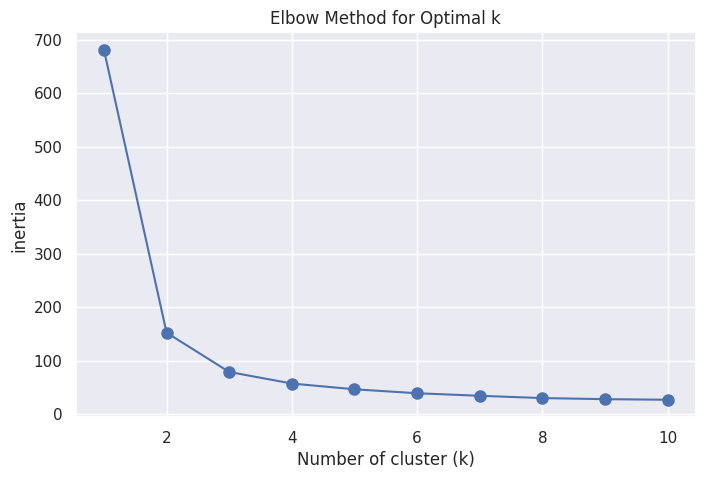
# 최적의 군집 개수 찾기
iris = load_iris()
X = iris.data
# 엘보우 기법 사용을 위해 KMeans() 모델 실행 및 inertia(중심점 거리의 제곱 합) 계산
# 엘보우 방식 : 클러스터 개수를 늘리면서 inertia의 변화를 관찰해 최적의 군집 개수를 찾는 방법
# 클러스터 개수를 증가 시킬때 inertia의 기울기가 완만해지는 지점 찾기
inertia_list = [] # 거리의 제곱 합 리스트 저장
k_values = range(1, 11) # 1부터 10개까지 군집 개수별 inertia 비교
for k in k_values:
kmeans = KMeans(n_clusters=k, random_state=123)
# random_state : 랜덤 초기 중심점 설정 시드, 동일한 시드에서 동일한 클러스터 수로 KMeans를 돌리면 항상 초기 중심점 위치는 같다
kmeans.fit(X) # 데이터 X를 사용하여 KMeans 모델 실행 → 최적의 클러스터 중심점 결과 도출
inertia_list.append(kmeans.inertia_) # 클러스터 갯수에 따른 inertia 저장
# 엘보우 기법 시각화
plt.figure(figsize = (8,5)) # 차트 사이즈
plt.plot(k_values, inertia_list, 'bo-', markersize=8) # b 파란색 o 원형마커 - 선스타일 그래프 지정
plt.xlabel('Number of cluster (k)')
plt.ylabel('inertia')
plt.title('Elbow Method for Optimal k')
plt.grid(True)
plt.show()
# 클러스터 수가 3개를 넘어가면 기울기가 완만해짐
1
2
3
4
5
6
7
8
9
10
11
12
13
14
15
16
17
18
19
20
/usr/local/lib/python3.10/dist-packages/sklearn/cluster/_kmeans.py:1416: FutureWarning: The default value of `n_init` will change from 10 to 'auto' in 1.4. Set the value of `n_init` explicitly to suppress the warning
  super()._check_params_vs_input(X, default_n_init=10)
/usr/local/lib/python3.10/dist-packages/sklearn/cluster/_kmeans.py:1416: FutureWarning: The default value of `n_init` will change from 10 to 'auto' in 1.4. Set the value of `n_init` explicitly to suppress the warning
  super()._check_params_vs_input(X, default_n_init=10)
/usr/local/lib/python3.10/dist-packages/sklearn/cluster/_kmeans.py:1416: FutureWarning: The default value of `n_init` will change from 10 to 'auto' in 1.4. Set the value of `n_init` explicitly to suppress the warning
  super()._check_params_vs_input(X, default_n_init=10)
/usr/local/lib/python3.10/dist-packages/sklearn/cluster/_kmeans.py:1416: FutureWarning: The default value of `n_init` will change from 10 to 'auto' in 1.4. Set the value of `n_init` explicitly to suppress the warning
  super()._check_params_vs_input(X, default_n_init=10)
/usr/local/lib/python3.10/dist-packages/sklearn/cluster/_kmeans.py:1416: FutureWarning: The default value of `n_init` will change from 10 to 'auto' in 1.4. Set the value of `n_init` explicitly to suppress the warning
  super()._check_params_vs_input(X, default_n_init=10)
/usr/local/lib/python3.10/dist-packages/sklearn/cluster/_kmeans.py:1416: FutureWarning: The default value of `n_init` will change from 10 to 'auto' in 1.4. Set the value of `n_init` explicitly to suppress the warning
  super()._check_params_vs_input(X, default_n_init=10)
/usr/local/lib/python3.10/dist-packages/sklearn/cluster/_kmeans.py:1416: FutureWarning: The default value of `n_init` will change from 10 to 'auto' in 1.4. Set the value of `n_init` explicitly to suppress the warning
  super()._check_params_vs_input(X, default_n_init=10)
/usr/local/lib/python3.10/dist-packages/sklearn/cluster/_kmeans.py:1416: FutureWarning: The default value of `n_init` will change from 10 to 'auto' in 1.4. Set the value of `n_init` explicitly to suppress the warning
  super()._check_params_vs_input(X, default_n_init=10)
/usr/local/lib/python3.10/dist-packages/sklearn/cluster/_kmeans.py:1416: FutureWarning: The default value of `n_init` will change from 10 to 'auto' in 1.4. Set the value of `n_init` explicitly to suppress the warning
  super()._check_params_vs_input(X, default_n_init=10)
/usr/local/lib/python3.10/dist-packages/sklearn/cluster/_kmeans.py:1416: FutureWarning: The default value of `n_init` will change from 10 to 'auto' in 1.4. Set the value of `n_init` explicitly to suppress the warning
  super()._check_params_vs_input(X, default_n_init=10)
1
2
3
4
5
6
7
8
9
10
11
12
13
14
15
16
17
18
19
20
21
22
23
24
25
26
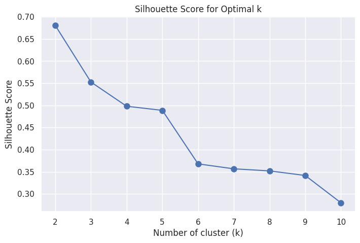
# 실루엣 계수 구하기
# 실루엣 계수 : 클러스터링 품질을 평가하기 위한 지표
from sklearn.metrics import silhouette_score
# 실루엣 계수 계산 및 시각화를 위한 KMeans 실행
silhouette_scores = []
k_values = range(2, 11)
for k in k_values:
kmeans = KMeans(n_clusters=k, random_state=123)
kmeans.fit(X)
labels = kmeans.labels_
score = silhouette_score(X, labels) # 각 k에 대한 실루엣 계수 저장
silhouette_scores.append(score)
# 실루엣 계수 시각화
plt.figure(figsize = (8,5))
plt.plot(k_values, silhouette_scores, 'bo-', markersize=8)
plt.xlabel('Number of cluster (k)')
plt.ylabel('Silhouette Score')
plt.title('Silhouette Score for Optimal k')
plt.grid(True)
plt.show()
# 엘보우 기법과 실루엣 계수를 종합적으로보면 클러스터 갯수가 2개일때 최적으로 보이나,
# 실제로 사용한 iris데이터는 3개의 서로 다른 품종으로 구성되어있어 클러스터 갯수가 3개일때 최적으로 보임
1
2
3
4
5
6
7
8
9
10
11
12
13
14
15
16
17
18
/usr/local/lib/python3.10/dist-packages/sklearn/cluster/_kmeans.py:1416: FutureWarning: The default value of `n_init` will change from 10 to 'auto' in 1.4. Set the value of `n_init` explicitly to suppress the warning
  super()._check_params_vs_input(X, default_n_init=10)
/usr/local/lib/python3.10/dist-packages/sklearn/cluster/_kmeans.py:1416: FutureWarning: The default value of `n_init` will change from 10 to 'auto' in 1.4. Set the value of `n_init` explicitly to suppress the warning
  super()._check_params_vs_input(X, default_n_init=10)
/usr/local/lib/python3.10/dist-packages/sklearn/cluster/_kmeans.py:1416: FutureWarning: The default value of `n_init` will change from 10 to 'auto' in 1.4. Set the value of `n_init` explicitly to suppress the warning
  super()._check_params_vs_input(X, default_n_init=10)
/usr/local/lib/python3.10/dist-packages/sklearn/cluster/_kmeans.py:1416: FutureWarning: The default value of `n_init` will change from 10 to 'auto' in 1.4. Set the value of `n_init` explicitly to suppress the warning
  super()._check_params_vs_input(X, default_n_init=10)
/usr/local/lib/python3.10/dist-packages/sklearn/cluster/_kmeans.py:1416: FutureWarning: The default value of `n_init` will change from 10 to 'auto' in 1.4. Set the value of `n_init` explicitly to suppress the warning
  super()._check_params_vs_input(X, default_n_init=10)
/usr/local/lib/python3.10/dist-packages/sklearn/cluster/_kmeans.py:1416: FutureWarning: The default value of `n_init` will change from 10 to 'auto' in 1.4. Set the value of `n_init` explicitly to suppress the warning
  super()._check_params_vs_input(X, default_n_init=10)
/usr/local/lib/python3.10/dist-packages/sklearn/cluster/_kmeans.py:1416: FutureWarning: The default value of `n_init` will change from 10 to 'auto' in 1.4. Set the value of `n_init` explicitly to suppress the warning
  super()._check_params_vs_input(X, default_n_init=10)
/usr/local/lib/python3.10/dist-packages/sklearn/cluster/_kmeans.py:1416: FutureWarning: The default value of `n_init` will change from 10 to 'auto' in 1.4. Set the value of `n_init` explicitly to suppress the warning
  super()._check_params_vs_input(X, default_n_init=10)
/usr/local/lib/python3.10/dist-packages/sklearn/cluster/_kmeans.py:1416: FutureWarning: The default value of `n_init` will change from 10 to 'auto' in 1.4. Set the value of `n_init` explicitly to suppress the warning
  super()._check_params_vs_input(X, default_n_init=10)
1
2
3
4
5
6
# 3개의 클러스터로 진행
from sklearn.cluster import KMeans

kmeans = KMeans(n_clusters=3, init='k-means++', max_iter=300, random_state=0)
kmeans.fit(iris_df)
1
2
/usr/local/lib/python3.10/dist-packages/sklearn/cluster/_kmeans.py:1416: FutureWarning: The default value of `n_init` will change from 10 to 'auto' in 1.4. Set the value of `n_init` explicitly to suppress the warning
  super()._check_params_vs_input(X, default_n_init=10)
KMeans(n_clusters=3, random_state=0)In a Jupyter environment, please rerun this cell to show the HTML representation or trust the notebook.
On GitHub, the HTML representation is unable to render, please try loading this page with nbviewer.org.
KMeans(n_clusters=3, random_state=0)
1
2
3
iris_df['target'] = iris.target   # 아이리스 데이터 포인트의 품종 정보
iris_df['cluster'] = kmeans.labels_  # 클러스터 위치
iris_df
| sepal length (cm) | sepal width (cm) | petal length (cm) | petal width (cm) | target | cluster | |
|---|---|---|---|---|---|---|
| 0 | 5.1 | 3.5 | 1.4 | 0.2 | 0 | 1 |
| 1 | 4.9 | 3.0 | 1.4 | 0.2 | 0 | 1 |
| 2 | 4.7 | 3.2 | 1.3 | 0.2 | 0 | 1 |
| 3 | 4.6 | 3.1 | 1.5 | 0.2 | 0 | 1 |
| 4 | 5.0 | 3.6 | 1.4 | 0.2 | 0 | 1 |
| ... | ... | ... | ... | ... | ... | ... |
| 145 | 6.7 | 3.0 | 5.2 | 2.3 | 2 | 2 |
| 146 | 6.3 | 2.5 | 5.0 | 1.9 | 2 | 0 |
| 147 | 6.5 | 3.0 | 5.2 | 2.0 | 2 | 2 |
| 148 | 6.2 | 3.4 | 5.4 | 2.3 | 2 | 2 |
| 149 | 5.9 | 3.0 | 5.1 | 1.8 | 2 | 0 |
150 rows × 6 columns
1
2
3
4
5
# target과 cluster 간의 그룹별 개수 확인
iris_result = iris_df.groupby(['target', 'cluster']).size()
iris_result

# target 0과 1은 적절하게 군집이 잘 형성됐으나, target 2는 군집이 나뉘어짐
| 0 | ||
|---|---|---|
| target | cluster | |
| 0 | 1 | 50 |
| 1 | 0 | 48 |
| 2 | 2 | |
| 2 | 0 | 14 |
| 2 | 36 |
1
2
3
4
5
6
7
8
9
# 성능평가 지표 사용
from sklearn.metrics import adjusted_rand_score

# KMeans로 예측한 클러스터 레이블과 실제 타겟 값을 비교하여 성능 평가
ari_score = adjusted_rand_score(iris_df['target'], iris_df['cluster'])
# ARI : 조정 랜드 지수, target과 cluster 열의 유사성을 정량화하여
# 클러스터링 결과가 실제 품종 정보를 얼마나 잘 반영하는지 확인
print(f"ARI (Adjusted Rand Index): {ari_score}")
# 1에 가까울수록 두 레이블 간의 일치도가 높다.
1
ARI (Adjusted Rand Index): 0.7302382722834697
1
2
3
4
5
6
7
8
9
10
11
12
13
14
15
16
17
18
19
20
21
22
23
24
25
26
27
28
29
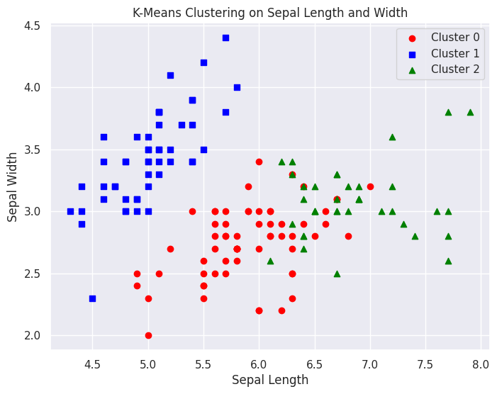
# sepal_length와 sepal_width로 산점도 시각화
import matplotlib.pyplot as plt
plt.figure(figsize = (8,6))
# cluster 값이 0, 1, 2 인 경우마다 다른 마커와 색상으로 시각화
plt.scatter(iris_df[iris_df['cluster'] == 0]['sepal length (cm)'],
iris_df[iris_df['cluster'] == 0]['sepal width (cm)'],
color='red', marker='o', label='Cluster 0')
plt.scatter(iris_df[iris_df['cluster'] == 1]['sepal length (cm)'],
iris_df[iris_df['cluster'] == 1]['sepal width (cm)'],
color='blue', marker='s', label='Cluster 1')
plt.scatter(iris_df[iris_df['cluster'] == 2]['sepal length (cm)'],
iris_df[iris_df['cluster'] == 2]['sepal width (cm)'],
color='green', marker='^', label='Cluster 2')
# 그래프의 제목과 축 설정
plt.title('K-Means Clustering on Sepal Length and Width')
plt.xlabel('Sepal Length')
plt.ylabel('Sepal Width')
# 범례 추가
plt.legend()
# 그래프 출력
plt.show()
# 뭔가 겹치는 구간들이 발생하고있다. 제대로 군집이 안되는 곳이 있다.
1
2
3
4
5
6
7
8
9
10
11
12
13
14
15
16
17
18
19
20
21
22
23
24
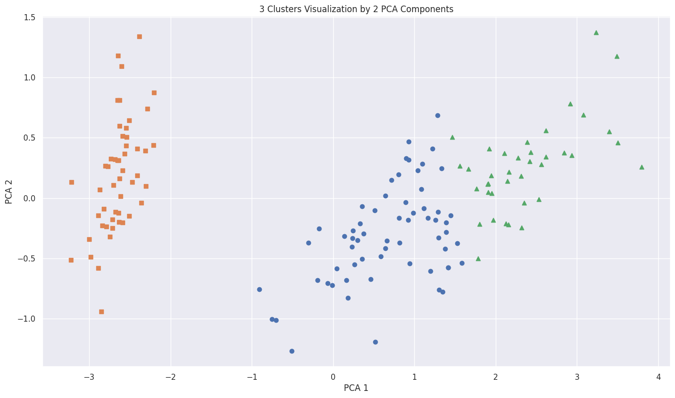
# iris 4개의 속성을 2차원 평면에 그리기 위해 PCA 2개로 차원 축소
# PCA : 고차원 데이터를 저차원으로 변환하는 기법
from sklearn.decomposition import PCA
pca = PCA(n_components=2) # 데이터를 2개의 주성분으로 축소
pca_transformed = pca.fit_transform(iris.data) # 주성분 출력
pca_transformed # 각 데이터 포인트가 2개의 주성분으로 표현된 새로운 배열
iris_df['pca_x'] = pca_transformed[:,0] # 첫 번째 주성분을 x열로
iris_df['pca_y'] = pca_transformed[:,1] # 두 번째 주성분을 y열로
# cluster 값이 0, 1, 2 인 경우마다 별도의 Index로 추출
marker0_ind = iris_df[iris_df['cluster']==0].index
marker1_ind = iris_df[iris_df['cluster']==1].index
marker2_ind = iris_df[iris_df['cluster']==2].index
# cluster값 0, 1, 2에 해당하는 Index로 각 cluster 레벨의 pca_x, pca_y 값 추출. o, s, ^ 로 marker 표시
plt.scatter(x=iris_df.loc[marker0_ind,'pca_x'], y=iris_df.loc[marker0_ind,'pca_y'], marker='o')
plt.scatter(x=iris_df.loc[marker1_ind,'pca_x'], y=iris_df.loc[marker1_ind,'pca_y'], marker='s')
plt.scatter(x=iris_df.loc[marker2_ind,'pca_x'], y=iris_df.loc[marker2_ind,'pca_y'], marker='^')
plt.xlabel('PCA 1')
plt.ylabel('PCA 2')
plt.title('3 Clusters Visualization by 2 PCA Components')
plt.show()
1
2
3
4
5
6
7
8
9
10
11
12
13
14
15
16
17
18
19
20
21
22
23
24
25
26
27
28
29
30
31
32
33
34
35
36
37
38
39
40
41
42
43
44
45
46
47
48
49
50
51
52
53
54
55
56
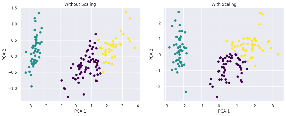
# 스케일링 후 진행 (스케일링 전후 비교)
from sklearn.preprocessing import StandardScaler
from sklearn.datasets import load_iris
from sklearn.cluster import KMeans
from sklearn.decomposition import PCA
import matplotlib.pyplot as plt
import pandas as pd
# 1. Iris 데이터 로드 및 DataFrame 변환
iris = load_iris()
irisDF = pd.DataFrame(data=iris.data, columns=['sepal_length', 'sepal_width', 'petal_length', 'petal_width'])
# 스케일링 적용하지 않은 경우
kmeans_no_scaling = KMeans(n_clusters=3, random_state=0)
kmeans_no_scaling.fit(irisDF)
irisDF['cluster_no_scaling'] = kmeans_no_scaling.labels_
# PCA로 차원 축소 (스케일링 하지 않은 데이터)
pca_no_scaling = PCA(n_components=2)
pca_transformed_no_scaling = pca_no_scaling.fit_transform(irisDF[['sepal_length', 'sepal_width', 'petal_length', 'petal_width']])
# 스케일링 적용
scaler = StandardScaler()
iris_scaled = scaler.fit_transform(irisDF[['sepal_length', 'sepal_width', 'petal_length', 'petal_width']])
# 스케일링 적용한 데이터로 KMeans 클러스터링
kmeans_with_scaling = KMeans(n_clusters=3, random_state=0)
kmeans_with_scaling.fit(iris_scaled)
irisDF['cluster_with_scaling'] = kmeans_with_scaling.labels_
# PCA로 차원 축소 (스케일링 한 데이터)
pca_with_scaling = PCA(n_components=2)
pca_transformed_with_scaling = pca_with_scaling.fit_transform(iris_scaled)
# 2개의 플롯을 그리기 위해 figure 생성
fig, ax = plt.subplots(1, 2, figsize=(14, 5))
# 스케일링 안 한 결과 시각화
ax[0].scatter(pca_transformed_no_scaling[:, 0], pca_transformed_no_scaling[:, 1],
c=irisDF['cluster_no_scaling'], cmap='viridis', marker='o')
# c : 데이터 포인트의 색상 지정, 각 클러스터마다 다른 색상 할당
# cmap : 색상 맵 지정, viridis(어두운 것에서 밝은 색상으로)
ax[0].set_title('Without Scaling')
ax[0].set_xlabel('PCA 1')
ax[0].set_ylabel('PCA 2')
# 스케일링 한 결과 시각화
ax[1].scatter(pca_transformed_with_scaling[:, 0], pca_transformed_with_scaling[:, 1],
c=irisDF['cluster_with_scaling'], cmap='viridis', marker='o')
ax[1].set_title('With Scaling')
ax[1].set_xlabel('PCA 1')
ax[1].set_ylabel('PCA 2')
plt.show()
# 스케일링을 하고나니 조금더 깔끔한 군집이 형성됨
1
2
3
4
/usr/local/lib/python3.10/dist-packages/sklearn/cluster/_kmeans.py:1416: FutureWarning: The default value of `n_init` will change from 10 to 'auto' in 1.4. Set the value of `n_init` explicitly to suppress the warning
  super()._check_params_vs_input(X, default_n_init=10)
/usr/local/lib/python3.10/dist-packages/sklearn/cluster/_kmeans.py:1416: FutureWarning: The default value of `n_init` will change from 10 to 'auto' in 1.4. Set the value of `n_init` explicitly to suppress the warning
  super()._check_params_vs_input(X, default_n_init=10)
1
2
3
4
5
6
7
8
9
10
11
12
13
14
15
16
17
18
19
20
21
22
23
24
25
26
27
28
29
30
31
32
33
34
35
36
37
38
39
40
41
42
43
44
45
46
47
48
49
50
51
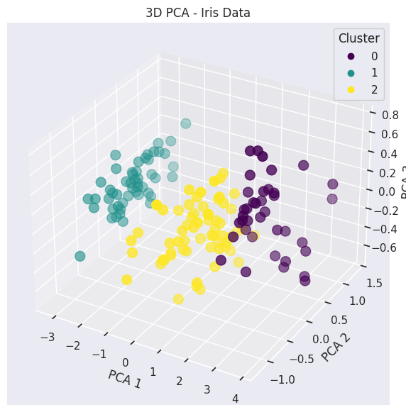
# 주성분 3개 적용
import pandas as pd
from sklearn.decomposition import PCA
from sklearn.cluster import KMeans
import matplotlib.pyplot as plt
from mpl_toolkits.mplot3d import Axes3D
from sklearn.datasets import load_iris
# 1. Iris 데이터 로드 및 DataFrame 변환
iris = load_iris()
irisDF = pd.DataFrame(data=iris.data, columns=['sepal_length', 'sepal_width', 'petal_length', 'petal_width'])
# 2. 데이터 스케일링
from sklearn.preprocessing import StandardScaler
scaler = StandardScaler()
iris_scaled = scaler.fit_transform(irisDF)
# 3. KMeans 클러스터링 수행
kmeans = KMeans(n_clusters=3, random_state=123)
kmeans.fit(irisDF)
irisDF['cluster'] = kmeans.labels_
# 4. PCA를 사용해 3개의 주성분으로 차원 축소
pca = PCA(n_components=3)
pca_transformed = pca.fit_transform(irisDF[['sepal_length', 'sepal_width', 'petal_length', 'petal_width']])
# 5. PCA 결과를 DataFrame에 추가
irisDF['pca_x'] = pca_transformed[:, 0]
irisDF['pca_y'] = pca_transformed[:, 1]
irisDF['pca_z'] = pca_transformed[:, 2]
# 6. 3D 시각화
fig = plt.figure(figsize=(10, 7))
ax = fig.add_subplot(111, projection='3d')
# 클러스터별로 색상 다르게 표시
scatter = ax.scatter(irisDF['pca_x'], irisDF['pca_y'], irisDF['pca_z'],
c=irisDF['cluster'], cmap='viridis', s=100)
# 축 및 그래프 설정
ax.set_xlabel('PCA 1')
ax.set_ylabel('PCA 2')
ax.set_zlabel('PCA 3')
ax.set_title('3D PCA - Iris Data')
# 컬러바 추가 (클러스터를 구분하기 위한 색상 범위)
legend1 = ax.legend(*scatter.legend_elements(), title="Cluster")
ax.add_artist(legend1)
plt.show()
1
2
/usr/local/lib/python3.10/dist-packages/sklearn/cluster/_kmeans.py:1416: FutureWarning: The default value of `n_init` will change from 10 to 'auto' in 1.4. Set the value of `n_init` explicitly to suppress the warning
  super()._check_params_vs_input(X, default_n_init=10)
1
2
3
4
5
6
7
8
9
10
11
12
13
14
15
16
17
18
19
20
21
22
23
24
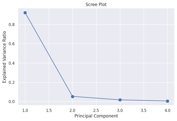
# 주성분 누적 기여율
# 1. 아이리스 데이터 로드
iris = load_iris()
irisDF = pd.DataFrame(data=iris.data, columns=['sepal_length', 'sepal_width', 'petal_length', 'petal_width'])
# 2. PCA 적용 (주성분 4개)
pca = PCA(n_components=4)
pca.fit(irisDF)
# 3. 각 주성분이 설명하는 분산의 비율 확인
explained_variance = pca.explained_variance_ratio_
print(f'각 주성분이 설명하는 분산 비율: {explained_variance}')
# 4. 첫 번째와 두 번째 주성분의 누적 분산 비율
cumulative_variance = explained_variance.cumsum() # 누적 분산 비율 계산
print(f'누적 분산 비율 (PCA 1~2): {cumulative_variance[1]}') # PCA 1 + PCA 2의 누적 비율
# 첫번째 주성분 : 데이터의 약 92%의 분산을 설명. 데이터의 변동성을 가장 잘 파악하고 있다
# 두번째 주성분 : 데이터의 약 5%의 분산을 설명. 첫번째 주성분에 비해 적은 비중을 파악하고 있다
# 세번째 네번째 주성분 : 데이터의 약 1.7%, 0.5%의 분산을 설명. 매우 적은 비중을 파악하고 있음
# 누적 분산 비율 : 첫번째와 두번째의 주성분만으로 원래 데이터의 97.7%의 정보를 유지할 수 있다.
# 따라서, 차원 축소를 통해 첫 번째와 두 번째 주성분만 사용하면 데이터의 대부분의 변동성을 설명할 수 있다.
# 결국, PCA를 통해 아이리스 데이터의 차원을 4차원에서 2차원으로 축소할 수 있고, 이 과정에서 데이터의 정보 손실이 매우 적다.
1
2
각 주성분이 설명하는 분산 비율: [0.92461872 0.05306648 0.01710261 0.00521218]
누적 분산 비율 (PCA 1~2): 0.977685206318795
1
2
3
4
5
6
7
8
9
10
11
12
13
14
15
16
17
18
19
20
21
22
23
24
25
26
27
28
import matplotlib.pyplot as plt
from sklearn.decomposition import PCA
from sklearn.datasets import load_iris

# 1. 아이리스 데이터 로드
iris = load_iris()
X = iris.data

# 2. PCA 수행 (주성분을 데이터의 모든 차원으로 설정)
pca = PCA(n_components=4)  # 아이리스 데이터는 4개의 차원을 가지고 있음
pca.fit(X)

# 3. 주성분이 설명하는 분산 비율
explained_variance_ratio = pca.explained_variance_ratio_

# 4. 스크리 플롯 시각화
plt.figure(figsize=(8, 5))
plt.plot(range(1, len(explained_variance_ratio) + 1), explained_variance_ratio, 'bo-', markersize=8)
plt.xlabel('Principal Component')
plt.ylabel('Explained Variance Ratio')
plt.title('Scree Plot')
plt.grid(True)
plt.show()

# 스크리 플롯 : 각 주성분이 데이터의 변동성을 얼마나 설명하는지를 시각적으로 표현
# 주성분 분석에서 몇 개의 주성분을 선택할지를 결정하는데 도움을 줌
# 스크리 플롯에서 설명된 분산 비율이 급격히 감소하는 지점(엘보우 포인트)을 찾아 그 지점까지의 주성분만을 선택하는 것이 일반적
문제풀어보기
1.데이터준비
1
2
3
4
5
6
import pandas as pd
pd.options.display.float_format = '{:,.2f}'.format

sales_df = pd.read_csv('/content/drive/MyDrive/sales_data.csv', index_col=['customer_id'])

sales_df
| total_buy_cnt | total_price | |
|---|---|---|
| customer_id | ||
| 12395 | 99 | 430250 |
| 12427 | 98 | 566410 |
| 12431 | 122 | 849900 |
| 12433 | 625 | 1180950 |
| 12471 | 10 | 97750 |
| ... | ... | ... |
| 18144 | 30 | 90750 |
| 18168 | 243 | 1533530 |
| 18225 | 1 | 91430 |
| 18229 | 48 | 559510 |
| 18239 | 230 | 1114480 |
254 rows × 2 columns
1
2
3
4
5
6
7
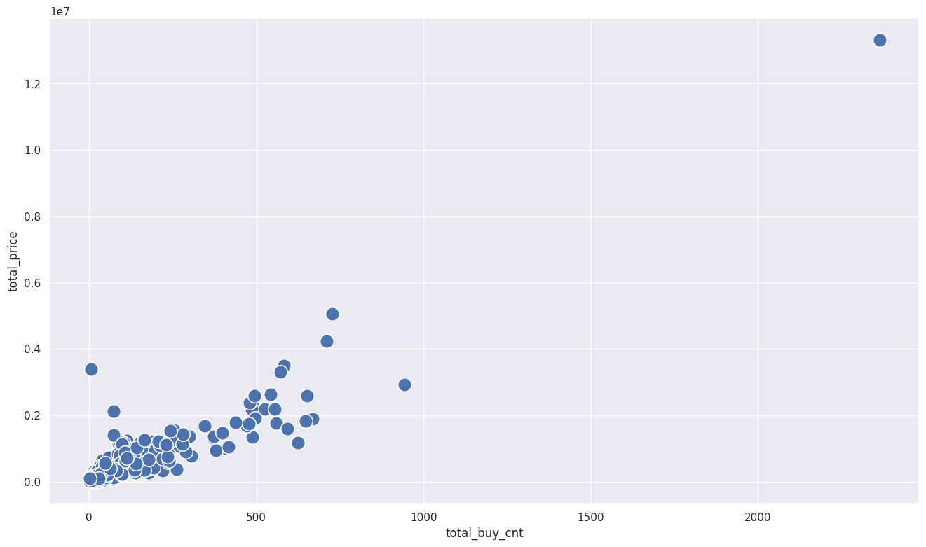
# 분포 확인하기
import seaborn as sns
sns.set(style='darkgrid', rc={'figure.figsize':(16,9)})
# 데이터 시각화
sns.scatterplot(x=sales_df['total_buy_cnt'], y=sales_df['total_price'], s=200)
# 이상치가 발견되었다.
1
<Axes: xlabel='total_buy_cnt', ylabel='total_price'>
1
2
3
4
5
6
7
8
9
10
11
12
13
14
15
16
17
18
19
20
21
22
23
24
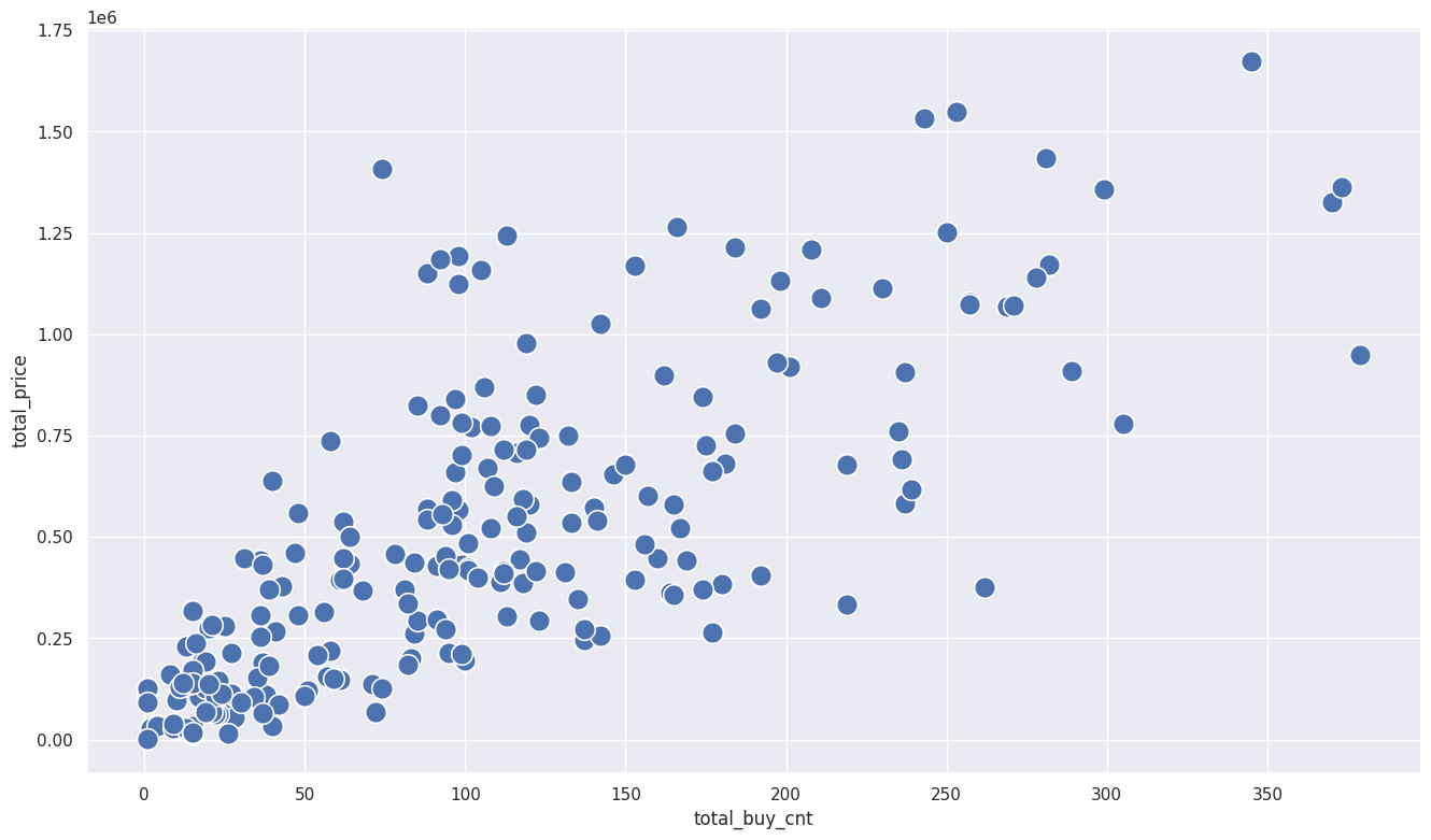
# 이상치 제거
def get_outlier_mask(df, weight=1.5):
Q1 = df.quantile(0.25)
Q3 = df.quantile(0.75)
IQR = Q3 - Q1
IQR_weight = IQR * weight
range_min = Q1 - IQR_weight
range_max = Q3 + IQR_weight
outlier_per_column = (df < range_min) | (df > range_max)
is_outlier = outlier_per_column.any(axis=1)
return is_outlier
outlier_idx_cust_df = get_outlier_mask(sales_df, weight=1.5)
# 이상치를 제거한 데이터 프레임만 추가
sales_df = sales_df[~outlier_idx_cust_df]
# 이상치를 제거한 데이터프레임 시각화
sns.scatterplot(x=sales_df['total_buy_cnt'], y=sales_df['total_price'], s=200)
1
<Axes: xlabel='total_buy_cnt', ylabel='total_price'>
1
2
3
4
5
6
7
8
9
10
11
12
13
14
15
# 값이 큰값들이 많아 표준화를 진행해보자

df_mean = sales_df.mean()  # 각 컬럼의 평균값
df_std = sales_df.std()  # 각 컬럼의 표준편차

scaled_df = (sales_df - df_mean)/df_std  # 컬럼별 표준화 진행

scaled_df.columns = ['total_buy_cnt', 'total_price']

# 인덱스 설정
scaled_df.index = sales_df.index

scaled_df
| total_buy_cnt | total_price | |
|---|---|---|
| customer_id | ||
| 12395 | -0.05 | -0.15 |
| 12427 | -0.07 | 0.21 |
| 12431 | 0.23 | 0.95 |
| 12471 | -1.13 | -1.02 |
| 12472 | -0.19 | 0.21 |
| ... | ... | ... |
| 18144 | -0.89 | -1.04 |
| 18168 | 1.69 | 2.74 |
| 18225 | -1.24 | -1.04 |
| 18229 | -0.67 | 0.19 |
| 18239 | 1.53 | 1.64 |
225 rows × 2 columns
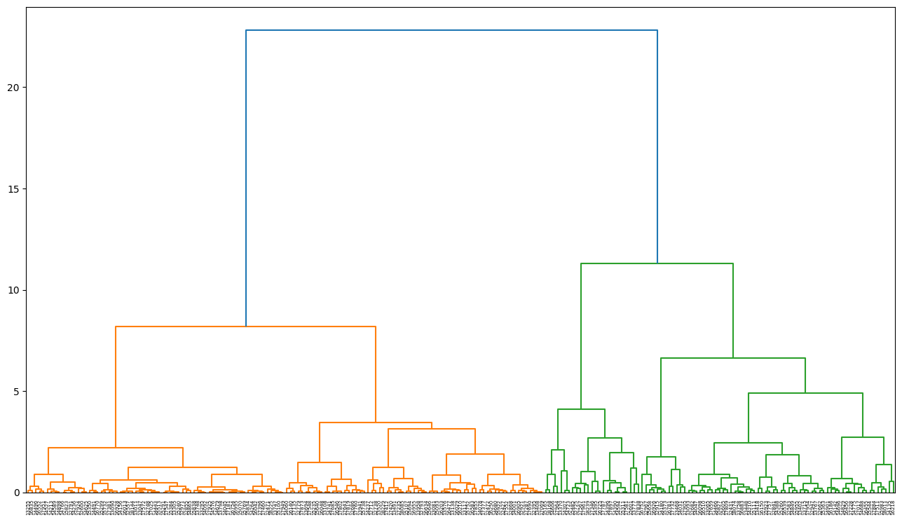
2.계층적 클러스터링
1
2
3
4
5
6
7
8
9
10
11
12
13
14
from scipy.cluster.hierarchy import dendrogram, linkage, cut_tree
import matplotlib.pyplot as plt

# 거리 : ward method 사용
model = linkage(scaled_df, 'ward')  # single, complete, average, centroid, median 등

labelList = scaled_df.index

# 덴드로그램 사이즈와 스타일 조정
plt.figure(figsize=(16,9))
plt.style.use("default")

dendrogram(model, labels=labelList)
plt.show()
1
2
3
4
5
6
7
cluster_num = 5

# 고객별 클러스터 라벨 구하기
scaled_df['label'] = cut_tree(model, cluster_num)

pd.DataFrame(scaled_df['label'].value_counts())
| count | |
|---|---|
| label | |
| 0 | 67 |
| 2 | 67 |
| 1 | 54 |
| 3 | 25 |
| 4 | 12 |
1
2
3
4
5
6
sns.set(style="darkgrid",
        rc = {'figure.figsize':(16,9)})

# 시각화
sns.scatterplot(x=scaled_df['total_price'], y=scaled_df['total_buy_cnt'], hue=scaled_df['label'], s=200, palette='bright')
1
<Axes: xlabel='total_price', ylabel='total_buy_cnt'>
3.K-Means
1
2
3
4
5
6
7
# k-means 클러스터링
from sklearn.cluster import KMeans
# k-means(k=2)
model = KMeans(n_clusters=2, random_state=123)
# 모델 학습
model.fit(scaled_df)
1
2
/usr/local/lib/python3.10/dist-packages/sklearn/cluster/_kmeans.py:1416: FutureWarning: The default value of `n_init` will change from 10 to 'auto' in 1.4. Set the value of `n_init` explicitly to suppress the warning
  super()._check_params_vs_input(X, default_n_init=10)
KMeans(n_clusters=2, random_state=123)In a Jupyter environment, please rerun this cell to show the HTML representation or trust the notebook.
On GitHub, the HTML representation is unable to render, please try loading this page with nbviewer.org.
KMeans(n_clusters=2, random_state=123)
1
2
3
4
5
6
# label 컬럼 생성
scaled_df['label'] = model.predict(scaled_df)

scaled_df
| total_buy_cnt | total_price | label | |
|---|---|---|---|
| customer_id | |||
| 12395 | -0.05 | -0.15 | 1 |
| 12427 | -0.07 | 0.21 | 1 |
| 12431 | 0.23 | 0.95 | 1 |
| 12471 | -1.13 | -1.02 | 1 |
| 12472 | -0.19 | 0.21 | 1 |
| ... | ... | ... | ... |
| 18144 | -0.89 | -1.04 | 1 |
| 18168 | 1.69 | 2.74 | 0 |
| 18225 | -1.24 | -1.04 | 1 |
| 18229 | -0.67 | 0.19 | 1 |
| 18239 | 1.53 | 1.64 | 0 |
225 rows × 3 columns
1
2
3
4
5
6
7
# 시각화
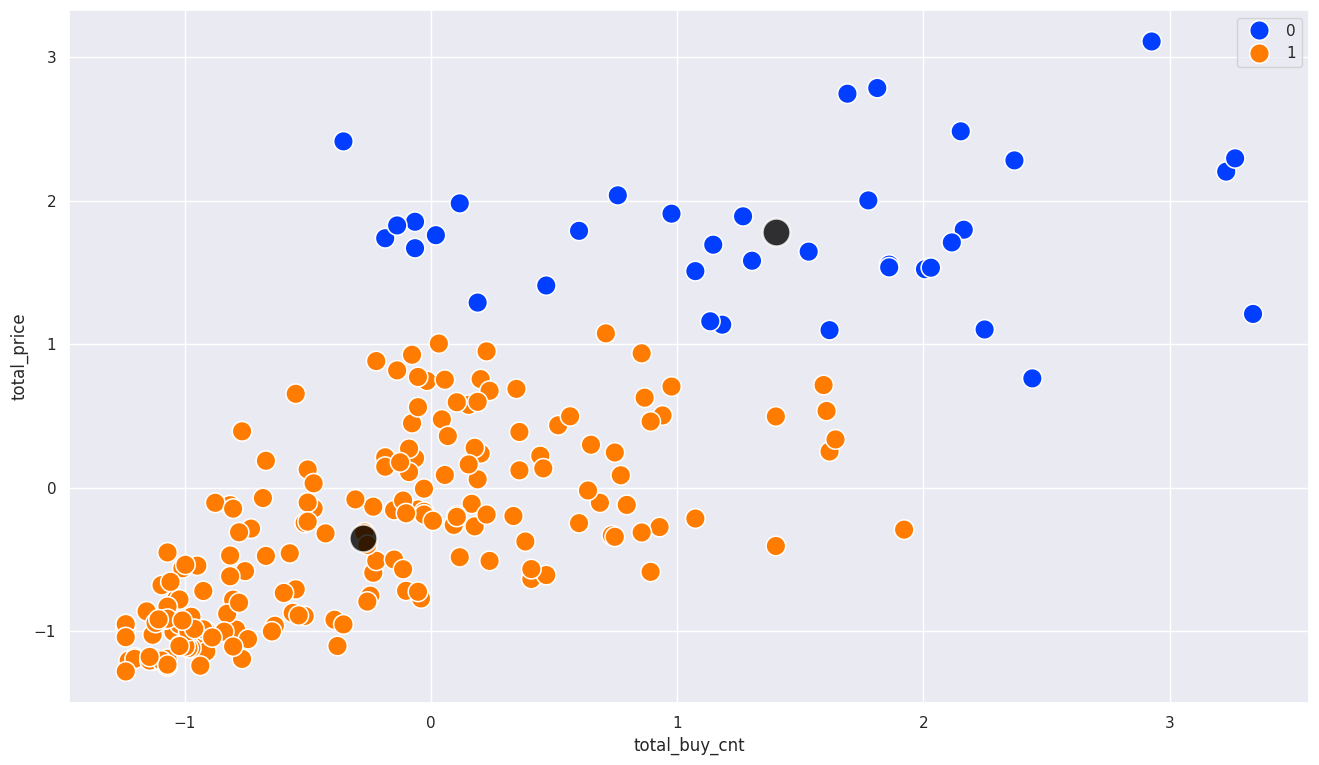
# 각 군집의 중심점
centers = model.cluster_centers_
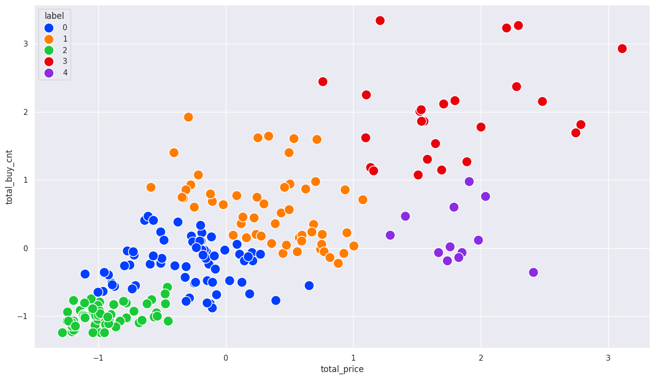
sns.scatterplot(x=scaled_df['total_buy_cnt'], y=scaled_df['total_price'], hue=scaled_df['label'], s=200, palette='bright')
sns.scatterplot(x=centers[:,0], y=centers[:,1], color='black', alpha=0.8, s=400)
1
<Axes: xlabel='total_buy_cnt', ylabel='total_price'>
1
2
3
# inertia 값 확인
print(model.inertia_)
1
362.10916862276144
1
2
3
4
5
6
# 이너시아 값 상대 비교

# scaled_df에 추가했던 label 열을 제거
scaled_df = scaled_df.drop(['label'], axis=1)
1
2
3
4
5
6
7
8
9
10
11
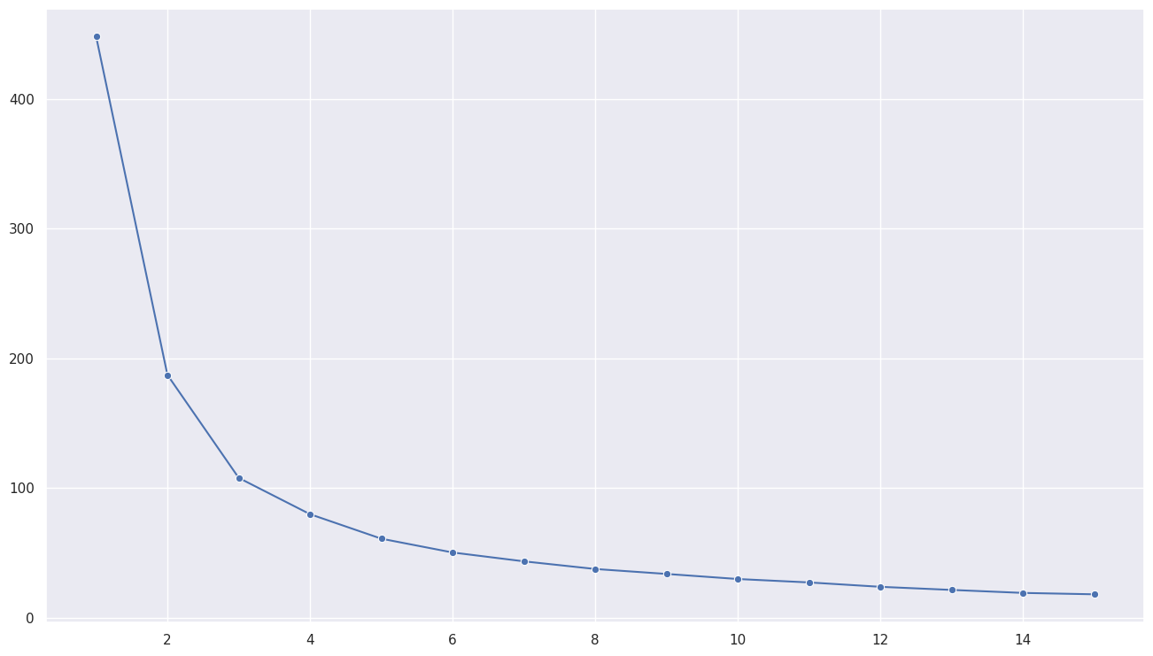
# inertia 값 저장할 리스트
inertias = []
for k in range(1, 16): # k값의 범위 1~15로 지정
model = KMeans(n_clusters=k, random_state=123)
model.fit(scaled_df)
inertias.append(model.inertia_)
# k값에 따른 inertia값 시각화
sns.lineplot(x=range(1, 16), y=inertias, marker='o')
1
2
3
4
5
6
7
8
9
10
11
12
13
14
15
16
17
18
19
20
21
22
23
24
25
26
27
28
29
30
31
32
33
34
35
36
/usr/local/lib/python3.10/dist-packages/sklearn/cluster/_kmeans.py:1416: FutureWarning: The default value of `n_init` will change from 10 to 'auto' in 1.4. Set the value of `n_init` explicitly to suppress the warning
  super()._check_params_vs_input(X, default_n_init=10)
/usr/local/lib/python3.10/dist-packages/sklearn/cluster/_kmeans.py:1416: FutureWarning: The default value of `n_init` will change from 10 to 'auto' in 1.4. Set the value of `n_init` explicitly to suppress the warning
  super()._check_params_vs_input(X, default_n_init=10)
/usr/local/lib/python3.10/dist-packages/sklearn/cluster/_kmeans.py:1416: FutureWarning: The default value of `n_init` will change from 10 to 'auto' in 1.4. Set the value of `n_init` explicitly to suppress the warning
  super()._check_params_vs_input(X, default_n_init=10)
/usr/local/lib/python3.10/dist-packages/sklearn/cluster/_kmeans.py:1416: FutureWarning: The default value of `n_init` will change from 10 to 'auto' in 1.4. Set the value of `n_init` explicitly to suppress the warning
  super()._check_params_vs_input(X, default_n_init=10)
/usr/local/lib/python3.10/dist-packages/sklearn/cluster/_kmeans.py:1416: FutureWarning: The default value of `n_init` will change from 10 to 'auto' in 1.4. Set the value of `n_init` explicitly to suppress the warning
  super()._check_params_vs_input(X, default_n_init=10)
/usr/local/lib/python3.10/dist-packages/sklearn/cluster/_kmeans.py:1416: FutureWarning: The default value of `n_init` will change from 10 to 'auto' in 1.4. Set the value of `n_init` explicitly to suppress the warning
  super()._check_params_vs_input(X, default_n_init=10)
/usr/local/lib/python3.10/dist-packages/sklearn/cluster/_kmeans.py:1416: FutureWarning: The default value of `n_init` will change from 10 to 'auto' in 1.4. Set the value of `n_init` explicitly to suppress the warning
  super()._check_params_vs_input(X, default_n_init=10)
/usr/local/lib/python3.10/dist-packages/sklearn/cluster/_kmeans.py:1416: FutureWarning: The default value of `n_init` will change from 10 to 'auto' in 1.4. Set the value of `n_init` explicitly to suppress the warning
  super()._check_params_vs_input(X, default_n_init=10)
/usr/local/lib/python3.10/dist-packages/sklearn/cluster/_kmeans.py:1416: FutureWarning: The default value of `n_init` will change from 10 to 'auto' in 1.4. Set the value of `n_init` explicitly to suppress the warning
  super()._check_params_vs_input(X, default_n_init=10)
/usr/local/lib/python3.10/dist-packages/sklearn/cluster/_kmeans.py:1416: FutureWarning: The default value of `n_init` will change from 10 to 'auto' in 1.4. Set the value of `n_init` explicitly to suppress the warning
  super()._check_params_vs_input(X, default_n_init=10)
/usr/local/lib/python3.10/dist-packages/sklearn/cluster/_kmeans.py:1416: FutureWarning: The default value of `n_init` will change from 10 to 'auto' in 1.4. Set the value of `n_init` explicitly to suppress the warning
  super()._check_params_vs_input(X, default_n_init=10)
/usr/local/lib/python3.10/dist-packages/sklearn/cluster/_kmeans.py:1416: FutureWarning: The default value of `n_init` will change from 10 to 'auto' in 1.4. Set the value of `n_init` explicitly to suppress the warning
  super()._check_params_vs_input(X, default_n_init=10)
/usr/local/lib/python3.10/dist-packages/sklearn/cluster/_kmeans.py:1416: FutureWarning: The default value of `n_init` will change from 10 to 'auto' in 1.4. Set the value of `n_init` explicitly to suppress the warning
  super()._check_params_vs_input(X, default_n_init=10)
/usr/local/lib/python3.10/dist-packages/sklearn/cluster/_kmeans.py:1416: FutureWarning: The default value of `n_init` will change from 10 to 'auto' in 1.4. Set the value of `n_init` explicitly to suppress the warning
  super()._check_params_vs_input(X, default_n_init=10)
/usr/local/lib/python3.10/dist-packages/sklearn/cluster/_kmeans.py:1416: FutureWarning: The default value of `n_init` will change from 10 to 'auto' in 1.4. Set the value of `n_init` explicitly to suppress the warning
  super()._check_params_vs_input(X, default_n_init=10)


<Axes: >
1
2
3
4
5
6
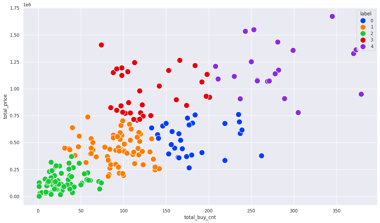
# k=5, 클러스터링 결과 해석
model = KMeans(n_clusters=5, random_state=123)
model.fit(scaled_df)
sales_df['label'] = model.predict(scaled_df) # 클러스터링만 진행
1
2
3
4
5
6
7
8
/usr/local/lib/python3.10/dist-packages/sklearn/cluster/_kmeans.py:1416: FutureWarning: The default value of `n_init` will change from 10 to 'auto' in 1.4. Set the value of `n_init` explicitly to suppress the warning
  super()._check_params_vs_input(X, default_n_init=10)
<ipython-input-94-0e3248d26b65>:5: SettingWithCopyWarning:
A value is trying to be set on a copy of a slice from a DataFrame.
Try using .loc[row_indexer,col_indexer] = value instead

See the caveats in the documentation: https://pandas.pydata.org/pandas-docs/stable/user_guide/indexing.html#returning-a-view-versus-a-copy
  sales_df['label'] = model.predict(scaled_df)  # 클러스터링만 진행
1
2
sns.scatterplot(x= sales_df['total_buy_cnt'], y= sales_df['total_price'], hue= sales_df['label'], s=200, palette='bright')
1
<Axes: xlabel='total_buy_cnt', ylabel='total_price'>
1
2
3
# 각 클러스터 고객 수 확인
pd.DataFrame(sales_df['label'].value_counts())
| count | |
|---|---|
| label | |
| 2 | 77 |
| 1 | 66 |
| 3 | 32 |
| 0 | 29 |
| 4 | 21 |
1
2
3
4
# 클러스터별 총 구매 금약과 구매 수량의 평균값

groupby_df = sales_df.groupby('label').mean()
groupby_df
| total_buy_cnt | total_price | |
|---|---|---|
| label | ||
| 0 | 181.14 | 536,495.17 |
| 1 | 91.79 | 432,910.30 |
| 2 | 25.64 | 127,196.23 |
| 3 | 127.78 | 963,223.12 |
| 4 | 280.33 | 1,192,478.57 |
1
2
3
4
5
6
# 평균 개당 가격 구하기
# 해석하기 (과제)

groupby_df['price_mean'] = groupby_df['total_price'] / groupby_df['total_buy_cnt']
groupby_df
| total_buy_cnt | total_price | price_mean | |
|---|---|---|---|
| label | |||
| 0 | 181.14 | 536,495.17 | 2,961.80 |
| 1 | 91.79 | 432,910.30 | 4,716.42 |
| 2 | 25.64 | 127,196.23 | 4,961.56 |
| 3 | 127.78 | 963,223.12 | 7,538.06 |
| 4 | 280.33 | 1,192,478.57 | 4,253.79 |
This post is licensed under CC BY 4.0 by the author.