파이썬 데이터분석 - 장바구니 분석(연관분석) 실습
- 고객의 정기예금 가입 여부 예측을 위한 은행 마케팅 분류 모델 구축
- 자전거 대여 수요 예측을 위한 머신러닝 모델 구축
- 파이썬 데이터분석 - A/B test 분석
- 파이썬 데이터분석 - aarrr 분석 실습
- 파이썬 데이터분석 - 장바구니 분석(연관분석)2 - FP-Growth, 순차패턴마이닝
- 파이썬 데이터분석 - 장바구니 분석(연관분석)
- 파이썬 데이터분석 데이터시각화 실습
- 파이썬 데이터분석 데이터시각화2
- 파이썬 데이터분석 데이터시각화1
- 파이썬 데이터분석 클러스터와 차원축소 실습
- 파이썬 데이터분석 클러스터와 차원축소2
- 파이썬 데이터분석 클러스터와 차원축소
- 파이썬 데이터분석 라이브러리
이번 미션에서는 베이커리 구매 데이터를 분석해볼 예정입니다. 사용할 데이터는 에든버러에 있는 베이커리의 고객 구매 데이터입니다. 이 데이터셋은 2016/1/11에서 2017/12/03까지 베이커리에서 제품을 구매한 고객들의 제품 구매 데이터입니다.
이 미션에서는 베이커리의 사장이라고 가정을 해보고, 고객의 구매 패턴을 분석하여 상품 간의 상호 작용이나 구매 행동의 흥미로운 패턴을 파악해 보아요. 데이터 EDA와 장바구니 분석을 적용하여 분석 결과를 도출해 봅시다. 이를 통해 베이커리의 매출을 증대시키고, 고객 만족도를 높이는 방법을 찾는 것이 목표입니다. 데이터 분석을 통해 어떤 전략이 효과적일지 아이디어를 얻어보세요.
1
2
3
4
5
6
### 개발환경 세팅하기

# ▶ 한글 폰트 다운로드
!sudo apt-get install -y fonts-nanum
!sudo fc-cache -fv
!rm ~/.cache/matplotlib -rf
1
2
3
4
5
6
7
8
9
10
11
12
13
14
15
16
17
18
19
20
21
Reading package lists... Done
Building dependency tree... Done
Reading state information... Done
fonts-nanum is already the newest version (20200506-1).
0 upgraded, 0 newly installed, 0 to remove and 49 not upgraded.
/usr/share/fonts: caching, new cache contents: 0 fonts, 1 dirs
/usr/share/fonts/truetype: caching, new cache contents: 0 fonts, 3 dirs
/usr/share/fonts/truetype/humor-sans: caching, new cache contents: 1 fonts, 0 dirs
/usr/share/fonts/truetype/liberation: caching, new cache contents: 16 fonts, 0 dirs
/usr/share/fonts/truetype/nanum: caching, new cache contents: 12 fonts, 0 dirs
/usr/local/share/fonts: caching, new cache contents: 0 fonts, 0 dirs
/root/.local/share/fonts: skipping, no such directory
/root/.fonts: skipping, no such directory
/usr/share/fonts/truetype: skipping, looped directory detected
/usr/share/fonts/truetype/humor-sans: skipping, looped directory detected
/usr/share/fonts/truetype/liberation: skipping, looped directory detected
/usr/share/fonts/truetype/nanum: skipping, looped directory detected
/var/cache/fontconfig: cleaning cache directory
/root/.cache/fontconfig: not cleaning non-existent cache directory
/root/.fontconfig: not cleaning non-existent cache directory
fc-cache: succeeded
1
2
3
4
5
6
7
8
9
10
11
12
# ▶ 한글 폰트 설정하기
import matplotlib.pyplot as plt
plt.rc('font', family='NanumBarunGothic')
plt.rcParams['axes.unicode_minus'] =False

# ▶ Warnings 제거
import warnings
warnings.filterwarnings('ignore')

# ▶ Google drive mount or 폴더 클릭 후 구글드라이브 연결
from google.colab import drive
drive.mount('/content/drive')
1
Drive already mounted at /content/drive; to attempt to forcibly remount, call drive.mount("/content/drive", force_remount=True).
1
2
import warnings
warnings.simplefilter('ignore')
1
2
3
4
5
6
7
8
9
10
11
12
13
14
##########################################
### 한글이 깨지는 경우 아래 코드 실행하기 !!!###
##########################################
import matplotlib.pyplot as plt
import matplotlib.font_manager as fm

# 나눔고딕 폰트를 설치합니다.
!apt-get install -y fonts-nanum
!fc-cache -fv

# 설치된 나눔고딕 폰트를 matplotlib에 등록합니다.
font_path = '/usr/share/fonts/truetype/nanum/NanumGothic.ttf'
fm.fontManager.addfont(font_path)
plt.rcParams['font.family'] = 'NanumGothic'
1
2
3
4
5
6
7
8
9
10
11
12
13
14
15
16
17
18
19
20
21
Reading package lists... Done
Building dependency tree... Done
Reading state information... Done
fonts-nanum is already the newest version (20200506-1).
0 upgraded, 0 newly installed, 0 to remove and 49 not upgraded.
/usr/share/fonts: caching, new cache contents: 0 fonts, 1 dirs
/usr/share/fonts/truetype: caching, new cache contents: 0 fonts, 3 dirs
/usr/share/fonts/truetype/humor-sans: caching, new cache contents: 1 fonts, 0 dirs
/usr/share/fonts/truetype/liberation: caching, new cache contents: 16 fonts, 0 dirs
/usr/share/fonts/truetype/nanum: caching, new cache contents: 12 fonts, 0 dirs
/usr/local/share/fonts: caching, new cache contents: 0 fonts, 0 dirs
/root/.local/share/fonts: skipping, no such directory
/root/.fonts: skipping, no such directory
/usr/share/fonts/truetype: skipping, looped directory detected
/usr/share/fonts/truetype/humor-sans: skipping, looped directory detected
/usr/share/fonts/truetype/liberation: skipping, looped directory detected
/usr/share/fonts/truetype/nanum: skipping, looped directory detected
/var/cache/fontconfig: cleaning cache directory
/root/.cache/fontconfig: not cleaning non-existent cache directory
/root/.fontconfig: not cleaning non-existent cache directory
fc-cache: succeeded
1
2
3
4
import os
import pandas as pd
import numpy as np
import seaborn as sns
데이터 준비하기
데이터 준비하기
데이터 출처: Kaggle
Bakery Sales Dataset데이터 설명
| 컬럼명 | 설명 |
|---|---|
| TransactionNo | 거래 ID |
| Items | 구매한 제품명 |
| DateTime | 거래 날짜 및 시각 |
| Daypart | 아침/오후/저녁/밤 중 언제 구매했는지 여부 |
| DayType | 주중/주말 중 언제 구매했는지 여부 |
데이터 전처리
1
pd.set_option('display.max_rows', 50)  # 모든 행을 표시하도록 설정
1
2
3
# 데이터 불러오기
df = pd.read_csv("/content/drive/MyDrive/Bakery.csv")
df
| TransactionNo | Items | DateTime | Daypart | DayType | |
|---|---|---|---|---|---|
| 0 | 1 | Bread | 2016.10.30 9:58 | Morning | Weekend |
| 1 | 2 | Scandinavian | 2016.10.30 10:05 | Morning | Weekend |
| 2 | 2 | Scandinavian | 2016.10.30 10:05 | Morning | Weekend |
| 3 | 3 | Hot chocolate | 2016.10.30 10:07 | Morning | Weekend |
| 4 | 3 | Jam | 2016.10.30 10:07 | Morning | Weekend |
| ... | ... | ... | ... | ... | ... |
| 20502 | 9682 | Coffee | 2017.9.4 14:32 | Afternoon | Weekend |
| 20503 | 9682 | Tea | 2017.9.4 14:32 | Afternoon | Weekend |
| 20504 | 9683 | Coffee | 2017.9.4 14:57 | Afternoon | Weekend |
| 20505 | 9683 | Pastry | 2017.9.4 14:57 | Afternoon | Weekend |
| 20506 | 9684 | Smoothies | 2017.9.4 15:04 | Afternoon | Weekend |
20507 rows × 5 columns
1
2
# 기본정보 확인
df.info()
1
2
3
4
5
6
7
8
9
10
11
12
<class 'pandas.core.frame.DataFrame'>
RangeIndex: 20507 entries, 0 to 20506
Data columns (total 5 columns):
 #   Column         Non-Null Count  Dtype
---  ------         --------------  -----
 0   TransactionNo  20507 non-null  int64
 1   Items          20507 non-null  object
 2   DateTime       20507 non-null  object
 3   Daypart        20507 non-null  object
 4   DayType        20507 non-null  object
dtypes: int64(1), object(4)
memory usage: 801.2+ KB
1
2
# 각 변수의 기술통계량 확인
df.describe(include='all')
| TransactionNo | Items | DateTime | Daypart | DayType | |
|---|---|---|---|---|---|
| count | 20507.000000 | 20507 | 20507 | 20507 | 20507 |
| unique | NaN | 94 | 9182 | 4 | 2 |
| top | NaN | Coffee | 2017.5.2 11:58 | Afternoon | Weekday |
| freq | NaN | 5471 | 12 | 11569 | 12807 |
| mean | 4976.202370 | NaN | NaN | NaN | NaN |
| std | 2796.203001 | NaN | NaN | NaN | NaN |
| min | 1.000000 | NaN | NaN | NaN | NaN |
| 25% | 2552.000000 | NaN | NaN | NaN | NaN |
| 50% | 5137.000000 | NaN | NaN | NaN | NaN |
| 75% | 7357.000000 | NaN | NaN | NaN | NaN |
| max | 9684.000000 | NaN | NaN | NaN | NaN |
중복값 처리
1
2
# 중복값 확인
df.duplicated().sum()
1
1620
1
2
3
# 중복값 내용 확인
duplicate_rows = df[df.duplicated(keep=False)]
print(duplicate_rows)
1
2
3
4
5
6
7
8
9
10
11
12
13
14
       TransactionNo         Items          DateTime    Daypart  DayType
1                  2  Scandinavian  2016.10.30 10:05    Morning  Weekend
2                  2  Scandinavian  2016.10.30 10:05    Morning  Weekend
23                11         Bread  2016.10.30 10:27    Morning  Weekend
25                11         Bread  2016.10.30 10:27    Morning  Weekend
48                21        Coffee  2016.10.30 10:49    Morning  Weekend
...              ...           ...               ...        ...      ...
20423           9634        Coffee    2017.8.4 16:30  Afternoon  Weekend
20464           9664        Coffee    2017.9.4 11:40    Morning  Weekend
20465           9664        Coffee    2017.9.4 11:40    Morning  Weekend
20472           9667      Sandwich    2017.9.4 12:04  Afternoon  Weekend
20473           9667      Sandwich    2017.9.4 12:04  Afternoon  Weekend

[3140 rows x 5 columns]
1
2
3
4
5
# 중복값 제거 : 똑같은걸 2개를 산건지 전산오류인지 수량의 정보가없어 확인할 방법이 없다. 본 분석에서는 중복값을 전부 제거하고 진행한다
print(f"중복값 제거 전 : {df.shape}")
df.drop_duplicates(inplace=True)
df.reset_index(drop=True, inplace=True)
print(f"중복값 제거 후 : {df.shape}")
1
2
중복값 제거 전 : (20507, 5)
중복값 제거 후 : (18887, 5)
1
2
# 중복값 확인
df.duplicated().sum()
1
0
결측치 처리
1
2
# 결측치 확인
df.isna().sum().sort_values(ascending=False)
| 0 | |
|---|---|
| TransactionNo | 0 |
| Items | 0 |
| DateTime | 0 |
| Daypart | 0 |
| DayType | 0 |
1
# 이상치는 특이사항 없는것으로 판단됐으나, 파생변수를 생성하면서 특이사항이 발견됨
파생변수 생성
1
2
3
4
5
6
7
8
9
10
11
12
13
14
15
# DateTime열을 년, 월, 요일, 시간으로 구분한다
# DateTime 변수를 datetime 형식으로 변환
df['DateTime'] = pd.to_datetime(df['DateTime'], format='%Y.%m.%d %H:%M')

# 파생변수 생성
df['Year'] = df['DateTime'].dt.year
df['Month'] = df['DateTime'].dt.month
df['Day'] = df['DateTime'].dt.day
df['DayOfWeek'] = df['DateTime'].dt.day_name()  # 요일
df['Hour'] = df['DateTime'].dt.hour

# 기존 DateTime 변수 제거
df.drop(columns=['DateTime'], inplace=True)

df
| TransactionNo | Items | Daypart | DayType | Year | Month | Day | DayOfWeek | Hour | |
|---|---|---|---|---|---|---|---|---|---|
| 0 | 1 | Bread | Morning | Weekend | 2016 | 10 | 30 | Sunday | 9 |
| 1 | 2 | Scandinavian | Morning | Weekend | 2016 | 10 | 30 | Sunday | 10 |
| 2 | 3 | Hot chocolate | Morning | Weekend | 2016 | 10 | 30 | Sunday | 10 |
| 3 | 3 | Jam | Morning | Weekend | 2016 | 10 | 30 | Sunday | 10 |
| 4 | 3 | Cookies | Morning | Weekend | 2016 | 10 | 30 | Sunday | 10 |
| ... | ... | ... | ... | ... | ... | ... | ... | ... | ... |
| 18882 | 9682 | Coffee | Afternoon | Weekend | 2017 | 9 | 4 | Monday | 14 |
| 18883 | 9682 | Tea | Afternoon | Weekend | 2017 | 9 | 4 | Monday | 14 |
| 18884 | 9683 | Coffee | Afternoon | Weekend | 2017 | 9 | 4 | Monday | 14 |
| 18885 | 9683 | Pastry | Afternoon | Weekend | 2017 | 9 | 4 | Monday | 14 |
| 18886 | 9684 | Smoothies | Afternoon | Weekend | 2017 | 9 | 4 | Monday | 15 |
18887 rows × 9 columns
이상치 처리
1
2
3
4
5
6
7
8
9
10
11
12
13
14
15
# 어라? 거래번호 9684는 DayType은 주말인데 DayOfWeek는 월요일이네? 이런데이터들이 얼마나 있을까?

# 조건 1: DayOfWeek가 일요일 또는 토요일인데 DayType이 'Weekend'가 아닌 데이터
condition1 = df[(df['DayOfWeek'].isin(['Saturday', 'Sunday'])) & (df['DayType'] != 'Weekend')]

# 조건 2: DayType이 'Weekend'인데 DayOfWeek가 일요일 또는 토요일이 아닌 데이터
condition2 = df[(df['DayType'] == 'Weekend') & (~df['DayOfWeek'].isin(['Saturday', 'Sunday']))]

# 결과
result1_count = condition1.shape[0]  # 조건 1의 수
result2_count = condition2.shape[0]  # 조건 2의 수

# 결과 출력
print(f"조건 1의 수: {result1_count}")
print(f"조건 2의 수: {result2_count}")
1
2
조건 1의 수: 955
조건 2의 수: 1882
1
df['DayType'].unique()
1
array(['Weekend', 'Weekday'], dtype=object)
1
df['Daypart'].unique()
1
array(['Morning', 'Afternoon', 'Evening', 'Night'], dtype=object)
1
2
3
4
5
# Daypart도 확인해볼필요가있다
# 각 Daypart별로 Hour의 고유값 확인
hour_by_daypart = df.groupby('Daypart')['Hour'].unique()

hour_by_daypart
| Hour | |
|---|---|
| Daypart | |
| Afternoon | [12, 13, 14, 15, 16] |
| Evening | [17, 18, 19, 20] |
| Morning | [9, 10, 11, 8, 7, 1] |
| Night | [21, 23, 22] |
1
2
3
4
5
# 아침인데 새벽1시 데이터만 수상해보인다
# Hour가 1인 데이터 필터링
hour_1_data = df[df['Hour'] == 1]

hour_1_data
| TransactionNo | Items | Daypart | DayType | Year | Month | Day | DayOfWeek | Hour | |
|---|---|---|---|---|---|---|---|---|---|
| 7594 | 4090 | Bread | Morning | Weekend | 2017 | 1 | 1 | Sunday | 1 |
이상치 처리방안
- 조건1 : ‘DayOfWeek’열에서 평일인데 ‘DayType’값이 ‘Weekend’라면 ‘Weekday’로 바꾼다
- 조건2 : ‘DayOfWeek’열에서 주말인데 ‘DayType’값이 ‘Weekday’라면 ‘Weekend’로 바꾼다
- 조건3 : ‘Hour’열에서 새벽1시인데 ‘Daypart’값이 ‘Morning’라면 ‘Night’로 바꾼다
1
2
3
4
5
6
7
8
9
10
11
12
13
14
15
16
17
18
19
20
21
22
23
24
25
26
27
28
29
30
31
# 이상치 처리

# 조건 1: 평일인데 DayType이 'Weekend'인 데이터 수 확인 및 변경
condition1 = df[(df['DayOfWeek'].isin(['Monday', 'Tuesday', 'Wednesday', 'Thursday', 'Friday'])) &
                 (df['DayType'] == 'Weekend')]
condition1_count = condition1.shape[0]  # 데이터 수

# 데이터 변경
df.loc[condition1.index, 'DayType'] = 'Weekday'

# 조건 2: 주말인데 DayType이 'Weekday'인 데이터 수 확인 및 변경
condition2 = df[(df['DayOfWeek'].isin(['Saturday', 'Sunday'])) &
                 (df['DayType'] == 'Weekday')]
condition2_count = condition2.shape[0]  # 데이터 수

# 데이터 변경
df.loc[condition2.index, 'DayType'] = 'Weekend'

# 조건 3: 새벽 1시인데 Daypart가 'Morning'인 데이터 수 확인 및 변경
condition3 = df[(df['Hour'] == 1) & (df['Daypart'] == 'Morning')]
condition3_count = condition3.shape[0]  # 데이터 수

# 데이터 변경
df.loc[condition3.index, 'Daypart'] = 'Night'

# 결과 출력
print(f"조건 1의 데이터 수: {condition1_count}")
print(f"조건 2의 데이터 수: {condition2_count}")
print(f"조건 3의 데이터 수: {condition3_count}")

df
1
2
3
조건 1의 데이터 수: 1882
조건 2의 데이터 수: 955
조건 3의 데이터 수: 1
| TransactionNo | Items | Daypart | DayType | Year | Month | Day | DayOfWeek | Hour | |
|---|---|---|---|---|---|---|---|---|---|
| 0 | 1 | Bread | Morning | Weekend | 2016 | 10 | 30 | Sunday | 9 |
| 1 | 2 | Scandinavian | Morning | Weekend | 2016 | 10 | 30 | Sunday | 10 |
| 2 | 3 | Hot chocolate | Morning | Weekend | 2016 | 10 | 30 | Sunday | 10 |
| 3 | 3 | Jam | Morning | Weekend | 2016 | 10 | 30 | Sunday | 10 |
| 4 | 3 | Cookies | Morning | Weekend | 2016 | 10 | 30 | Sunday | 10 |
| ... | ... | ... | ... | ... | ... | ... | ... | ... | ... |
| 18882 | 9682 | Coffee | Afternoon | Weekday | 2017 | 9 | 4 | Monday | 14 |
| 18883 | 9682 | Tea | Afternoon | Weekday | 2017 | 9 | 4 | Monday | 14 |
| 18884 | 9683 | Coffee | Afternoon | Weekday | 2017 | 9 | 4 | Monday | 14 |
| 18885 | 9683 | Pastry | Afternoon | Weekday | 2017 | 9 | 4 | Monday | 14 |
| 18886 | 9684 | Smoothies | Afternoon | Weekday | 2017 | 9 | 4 | Monday | 15 |
18887 rows × 9 columns
1
2
3
4
5
6
7
8
9
10
11
12
13
14
15
16
17
18
19
# 이상치가 처리됐는지 확인

# 조건 1: 평일인데 DayType이 'Weekend'인 데이터 수 확인
condition1 = df[(df['DayOfWeek'].isin(['Monday', 'Tuesday', 'Wednesday', 'Thursday', 'Friday'])) &
                 (df['DayType'] == 'Weekend')]
condition1_count = condition1.shape[0]  # 데이터 수

# 조건 2: 주말인데 DayType이 'Weekday'인 데이터 수 확인
condition2 = df[(df['DayOfWeek'].isin(['Saturday', 'Sunday'])) &
                 (df['DayType'] == 'Weekday')]
condition2_count = condition2.shape[0]  # 데이터 수

# 조건 3: 새벽 1시인데 Daypart가 'Morning'인 데이터 수 확인
condition3 = df[(df['Hour'] == 1) & (df['Daypart'] == 'Morning')]
condition3_count = condition3.shape[0]  # 데이터 수

print(f"조건 1의 데이터 수: {condition1_count}")
print(f"조건 2의 데이터 수: {condition2_count}")
print(f"조건 3의 데이터 수: {condition3_count}")
1
2
3
조건 1의 데이터 수: 0
조건 2의 데이터 수: 0
조건 3의 데이터 수: 0
EDA
1
2
# 각 변수의 기술통계량 확인
df.describe(include='all')
| TransactionNo | Items | Daypart | DayType | Year | Month | Day | DayOfWeek | Hour | |
|---|---|---|---|---|---|---|---|---|---|
| count | 18887.000000 | 18887 | 18887 | 18887 | 18887.000000 | 18887.000000 | 18887.000000 | 18887 | 18887.000000 |
| unique | NaN | 94 | 4 | 2 | NaN | NaN | NaN | 7 | NaN |
| top | NaN | Coffee | Afternoon | Weekday | NaN | NaN | NaN | Saturday | NaN |
| freq | NaN | 4528 | 10687 | 12757 | NaN | NaN | NaN | 3274 | NaN |
| mean | 4951.051517 | NaN | NaN | NaN | 2016.597924 | 6.047016 | 14.948589 | NaN | 12.276116 |
| std | 2811.619306 | NaN | NaN | NaN | 0.490330 | 4.141418 | 9.272868 | NaN | 2.342972 |
| min | 1.000000 | NaN | NaN | NaN | 2016.000000 | 1.000000 | 1.000000 | NaN | 1.000000 |
| 25% | 2496.500000 | NaN | NaN | NaN | 2016.000000 | 2.000000 | 4.000000 | NaN | 10.000000 |
| 50% | 5082.000000 | NaN | NaN | NaN | 2017.000000 | 5.000000 | 15.000000 | NaN | 12.000000 |
| 75% | 7378.500000 | NaN | NaN | NaN | 2017.000000 | 11.000000 | 23.000000 | NaN | 14.000000 |
| max | 9684.000000 | NaN | NaN | NaN | 2017.000000 | 12.000000 | 31.000000 | NaN | 23.000000 |
1
2
# 무엇이 많이 팔렸나
df['Items'].value_counts().head(20)
| count | |
|---|---|
| Items | |
| Coffee | 4528 |
| Bread | 3097 |
| Tea | 1350 |
| Cake | 983 |
| Pastry | 815 |
| Sandwich | 680 |
| Medialuna | 585 |
| Hot chocolate | 552 |
| Cookies | 515 |
| Brownie | 379 |
| Farm House | 371 |
| Juice | 365 |
| Muffin | 364 |
| Alfajores | 344 |
| Scone | 327 |
| Soup | 326 |
| Toast | 318 |
| Scandinavian | 275 |
| Truffles | 192 |
| Coke | 184 |
1
2
3
4
5
6
7
8
9
10
11
12
13
14
15
16
17
18
19
20
21
22
23
24
25
26
27
28
29
30
31
32
33
34
35
36
37
38
39
40
41
42
# 상위20개 하위20개 아이템 비율로 시각화하기

# 아이템별 판매량 계산
item_counts = df['Items'].value_counts()

# 전체 판매량 계산
total_sales = item_counts.sum()

# 비율 계산
item_ratios = (item_counts / total_sales) * 100

# 상위 20
top_items = item_ratios.nlargest(20).sort_values(ascending=True)

# 하위 20
bottom_items = item_ratios.nsmallest(20).sort_values(ascending=False)

# 서브플롯 생성
fig, axes = plt.subplots(1, 2, figsize=(12, 5))

# 상위20 아이템 시각화
top_items.plot(kind='barh', ax=axes[0], color='skyblue')
axes[0].set_title('Top 20 Best Selling Items by Percentage')
axes[0].set_ylabel('')
axes[0].spines[['top','right']].set_visible(False)

# 막대 옆에 비율 표시
for index, value in enumerate(top_items):
    axes[0].text(value, index, f'{value:.1f}%', va='center')

# 하위20 아이템 시각화
bottom_items.plot(kind='barh', ax=axes[1], color='salmon')
axes[1].set_title('Bottom 20 Selling Items by Percentage')
axes[1].set_ylabel('')
axes[1].spines[['top','right']].set_visible(False)

# 막대 옆에 비율 표시
for index, value in enumerate(bottom_items):
    axes[1].text(value, index, f'{value:.3f}%', va='center')

plt.tight_layout()
plt.show()
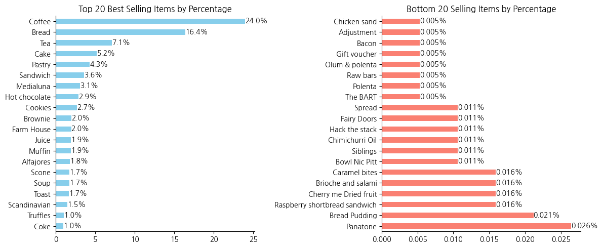
- 상위 판매 아이템 : 커피, 빵, 차, 케이크, 페이스트리 등이 잘나간다.
- 하위 판매 아이템 : 베이컨, 폴렌타, 오일 등 일반적인 베이커리 메뉴가 아닌 제품들의 판매비중이 0.03% 미만으로 관찰되었다
1
2
3
# 아이템별 판매비중이 심각하게 차이난다. 전체 94종류에서 메뉴를 개선할 필요가 있다
print(f"전체대비 0.5%미만 판매된 아이템 : 총 {item_ratios[item_ratios < 0.5].shape[0]}종류({(item_ratios[item_ratios < 0.5].shape[0]/df['Items'].nunique())*100:.2f}%) ")
item_ratios[item_ratios < 0.5]
1
전체대비 0.5%미만 판매된 아이템 : 총 64종류(68.09%)
| count | |
|---|---|
| Items | |
| Frittata | 0.428866 |
| Smoothies | 0.407688 |
| Keeping It Local | 0.333563 |
| The Nomad | 0.307090 |
| Focaccia | 0.285911 |
| ... | ... |
| Bacon | 0.005295 |
| Gift voucher | 0.005295 |
| Olum & polenta | 0.005295 |
| Raw bars | 0.005295 |
| Polenta | 0.005295 |
64 rows × 1 columns
- 2년동안 판매한 베이커리 아이템중에 0.5% 미만 판매된 아이템이 64종류나있고 전체중 68%를 차지한다.
- 즉, 판매하고있는아이템 2/3가 상품가치가 떨어지고 메뉴를 간소화하는 방안을 고민할 필요가있다
1
2
3
4
5
6
7
8
9
10
11
12
13
14
15
16
17
18
19
20
21
22
23
24
25
# 년도별 월별 판매수를 알아보자

# 월별 아이템 판매 수 집계
monthly_sales = df.groupby(['Year', 'Month']).size().unstack(fill_value=0)


fig, axes = plt.subplots(nrows=1, ncols=2, figsize=(12, 6), sharey=True)

# 2016년 판매 수 시각화
monthly_sales.loc[2016].plot(kind='bar', ax=axes[0], color='skyblue')
axes[0].set_title('2016년 월별 판매수')
axes[0].set_xlabel('')
axes[0].set_ylabel('')
axes[0].set_xticklabels(monthly_sales.columns, rotation=0)

# 2017년 판매 수 시각화
monthly_sales.loc[2017].plot(kind='bar', ax=axes[1], color='skyblue')
axes[1].set_title('2017년 월별 판매수')
axes[1].set_xlabel('')
axes[1].set_xticklabels(monthly_sales.columns, rotation=0)

# 레이아웃 조정
plt.tight_layout()
plt.show()
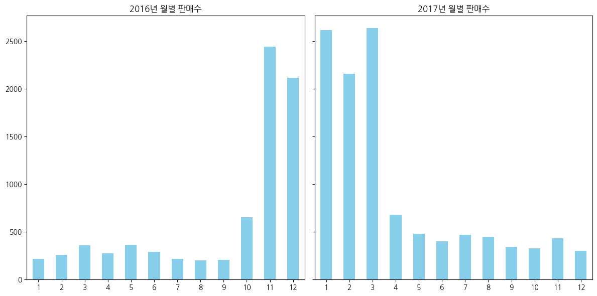
- 2016년 11월 ~ 2017년 3월 까지 판매량이 많았는데 그 이후로 판매량이 저조하다
- 겨울이 성수기라면, 2016년 1월 ~ 2016년 3월, 2017년 11월 ~ 2017년 12월 판매량은 왜 적을까?
1
2
3
4
5
6
7
8
9
10
11
12
13
14
15
16
17
18
19
20
21
22
23
24
25
26
27
28
29
30
31
32
33
34
35
# 년도별 월별 매장운영일수 확인

# 운영일수 집계 (중복된 날짜를 제외하기 위해 unique count)
operating_days = df.groupby(['Year', 'Month'])['Day'].nunique().unstack(fill_value=0)

# 서브플롯 생성
fig, axes = plt.subplots(nrows=1, ncols=2, figsize=(12, 6), sharey=True)

# 2016년 운영일수 시각화
bars_2016 = operating_days.loc[2016].plot(kind='bar', ax=axes[0], color='purple')
axes[0].set_title('2016년 월별 매장 운영일수')
axes[0].set_xlabel('')
axes[0].set_ylabel('운영일수')
axes[0].set_xticklabels(operating_days.columns, rotation=0)

# 막대 위에 숫자 표시
for bar in bars_2016.patches:
    axes[0].text(bar.get_x() + bar.get_width() / 2, bar.get_height(),
                  int(bar.get_height()), ha='center', va='bottom')

# 2017년 운영일수 시각화
bars_2017 = operating_days.loc[2017].plot(kind='bar', ax=axes[1], color='purple')
axes[1].set_title('2017년 월별 매장 운영일수')
axes[1].set_xlabel('')
axes[1].set_ylabel('운영일수')
axes[1].set_xticklabels(operating_days.columns, rotation=0)

# 막대 위에 숫자 표시
for bar in bars_2017.patches:
    axes[1].text(bar.get_x() + bar.get_width() / 2, bar.get_height(),
                  int(bar.get_height()), ha='center', va='bottom')

# 레이아웃 조정
plt.tight_layout()
plt.show()
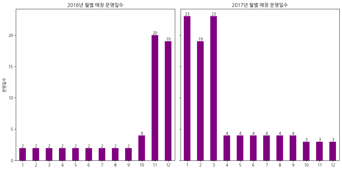
- 성수기 비수기 차이가아니라 일을안한게 문제였다
1
2
3
4
5
6
7
for i in range(1, 13):
    mask111 = df[(df['Year'].isin([2016])) & (df['Month'].isin([i]))]
    print(f"2016년 {i}월 매장운영일 : {mask111['Day'].unique()}")

for i in range(1, 13):
    mask111 = df[(df['Year'].isin([2017])) & (df['Month'].isin([i]))]
    print(f"2017년 {i}월 매장운영일 : {mask111['Day'].unique()}")
1
2
3
4
5
6
7
8
9
10
11
12
13
14
15
16
17
18
19
20
21
22
23
24
2016년 1월 매장운영일 : [11 12]
2016년 2월 매장운영일 : [11 12]
2016년 3월 매장운영일 : [11 12]
2016년 4월 매장운영일 : [11 12]
2016년 5월 매장운영일 : [11 12]
2016년 6월 매장운영일 : [11 12]
2016년 7월 매장운영일 : [11 12]
2016년 8월 매장운영일 : [11 12]
2016년 9월 매장운영일 : [11 12]
2016년 10월 매장운영일 : [30 31 11 12]
2016년 11월 매장운영일 : [11 13 14 15 16 17 18 19 20 21 22 23 24 25 26 27 28 29 30 12]
2016년 12월 매장운영일 : [11 12 13 14 15 16 17 18 19 20 21 22 23 24 27 28 29 30 31]
2017년 1월 매장운영일 : [ 1 13 14 15 16 17 18 19 20 21 22 23 24 25 26 27 28 29 30 31  2  3  4]
2017년 2월 매장운영일 : [ 2 13 14 15 16 17 18 19 20 21 22 23 24 25 26 27 28  3  4]
2017년 3월 매장운영일 : [ 1  2  3 13 14 15 16 17 18 19 20 21 22 23 24 25 26 27 28 29 30 31  4]
2017년 4월 매장운영일 : [1 2 3 4]
2017년 5월 매장운영일 : [1 2 3 4]
2017년 6월 매장운영일 : [1 2 3 4]
2017년 7월 매장운영일 : [1 2 3 4]
2017년 8월 매장운영일 : [1 2 3 4]
2017년 9월 매장운영일 : [1 2 3 4]
2017년 10월 매장운영일 : [1 2 3]
2017년 11월 매장운영일 : [1 2 3]
2017년 12월 매장운영일 : [1 2 3]
1
2
3
4
5
6
7
8
9
10
11
12
13
14
15
16
17
18
19
20
21
22
23
24
25
26
27
28
29
30
31
32
33
34
35
36
37
38
39
40
41
# 년도별 월별 매장운영일수 대비 판매수 확인

# 판매수 집계
monthly_sales = df.groupby(['Year', 'Month']).size().unstack(fill_value=0)

# 운영일수 집계 (중복된 날짜를 제외하기 위해 unique count)
operating_days = df.groupby(['Year', 'Month'])['Day'].nunique().unstack(fill_value=0)

# 월별 하루 평균 판매수 계산
average_sales_per_day = monthly_sales.div(operating_days)

# 서브플롯 생성
fig, axes = plt.subplots(nrows=1, ncols=2, figsize=(12, 6), sharey=True)

# 2016년 월별 판매수 대비 운영일수 시각화
average_sales_per_day.loc[2016].plot(kind='bar', ax=axes[0], color='skyblue')
axes[0].set_title('2016년 월별 하루 평균 판매수')
axes[0].set_xlabel('')
axes[0].set_ylabel('하루 평균 판매수')
axes[0].set_xticklabels(average_sales_per_day.columns, rotation=0)

# 막대 위에 숫자 표시
for bar in axes[0].patches:
    axes[0].text(bar.get_x() + bar.get_width() / 2, bar.get_height(),
                  f'{bar.get_height():.0f}', ha='center', va='bottom')

# 2017년 월별 판매수 대비 운영일수 시각화
average_sales_per_day.loc[2017].plot(kind='bar', ax=axes[1], color='skyblue')
axes[1].set_title('2017년 월별 하루 평균 판매수')
axes[1].set_xlabel('')
axes[1].set_ylabel('하루 평균 판매수')
axes[1].set_xticklabels(average_sales_per_day.columns, rotation=0)

# 막대 위에 숫자 표시
for bar in axes[1].patches:
    axes[1].text(bar.get_x() + bar.get_width() / 2, bar.get_height(),
                  f'{bar.get_height():.0f}', ha='center', va='bottom')

# 레이아웃 조정
plt.tight_layout()
plt.show()
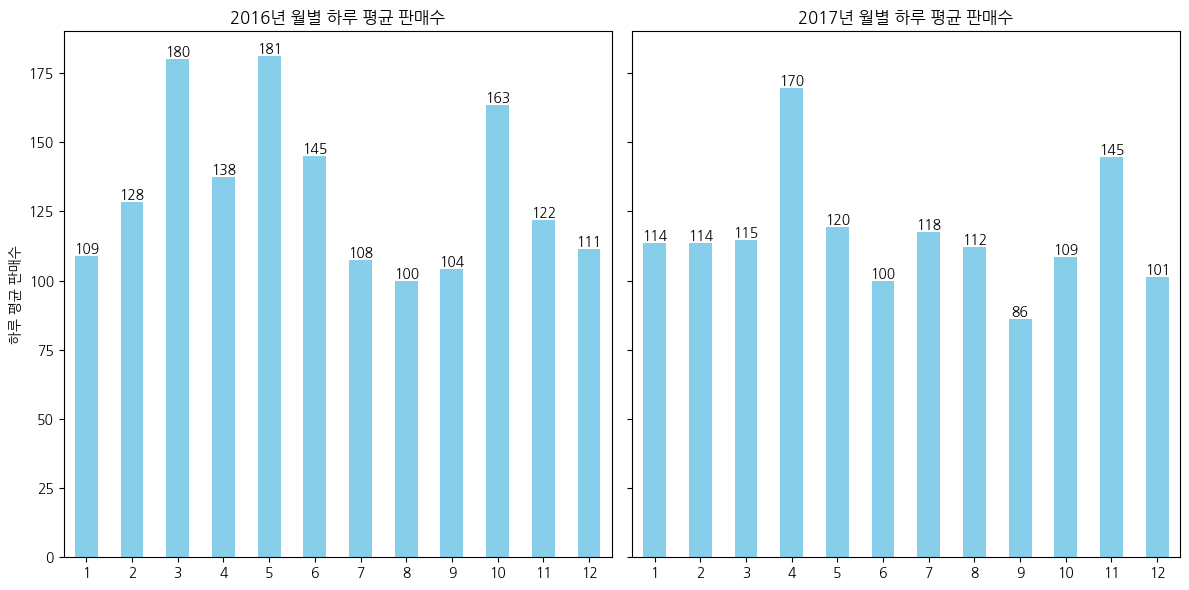
- 평균적으로 월별 하루 판매수는 100개 이상이고, 일부 달에는 평균보다 2배이상 판매를 하고있지만 대부분의 매장운영일수가 월별 4일 이하로 데이터가 부족하다
- 현재 데이터상으로는 하루 판매수를 일정하다고 간주할 수 있다
1
df['Daypart'].unique()
1
array(['Morning', 'Afternoon', 'Evening', 'Night'], dtype=object)
1
2
3
4
5
6
7
8
9
10
11
12
13
14
15
16
17
18
19
20
# 시간대별 판매수 확인

# 판매수 집계
daypart_sales = df['Daypart'].value_counts()

# 시각화
plt.figure(figsize=(8, 5))
daypart_sales.plot(kind='bar', color='skyblue')
plt.title('Daypart별 판매수')
plt.xlabel('Daypart')
plt.ylabel('판매수')
plt.xticks(rotation=0)

# 막대 위에 숫자 표시
for index, value in enumerate(daypart_sales):
    plt.text(index, value, str(value), ha='center', va='bottom')

# 그래프 표시
plt.tight_layout()
plt.show()
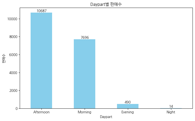
- 아침과 오후에 판매량이 압도적으로 많다
1
2
3
4
5
6
7
8
9
10
11
12
13
14
15
16
17
18
19
20
21
22
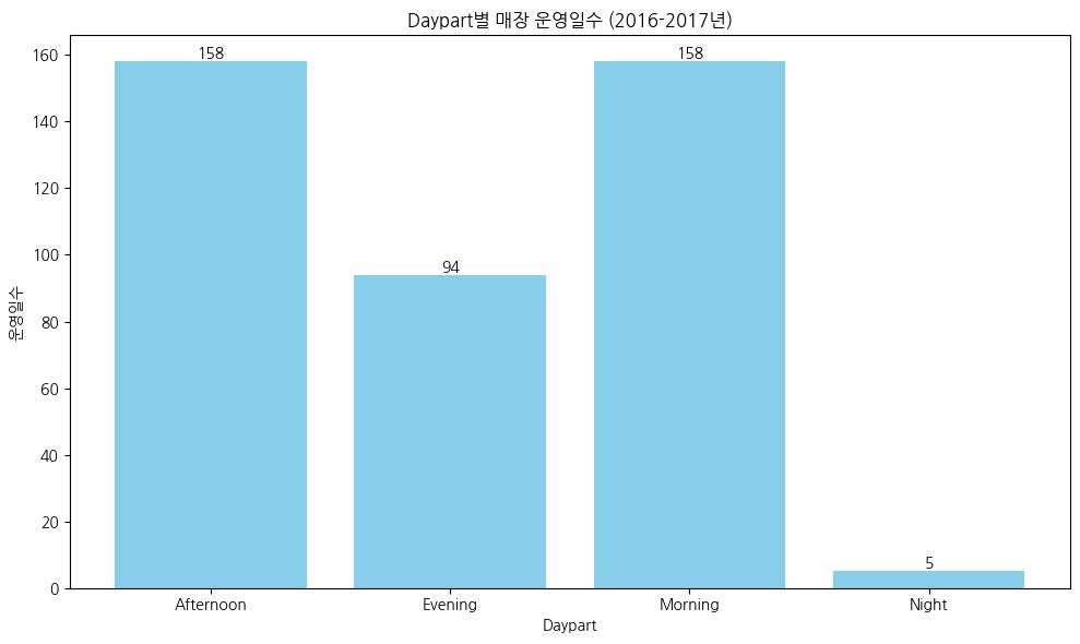
# 시간대별 매장운영일수 확인
# 운영일수 집계 (Daypart별로 Year, Month, Day가 중복되지 않도록)
operating_days = df.groupby(['Daypart', 'Year', 'Month', 'Day']).size().reset_index(name='Count')
# Daypart별 운영일수 계산
total_operating_days = operating_days.groupby('Daypart').size().reset_index(name='Operating Days')
# 시각화
plt.figure(figsize=(10, 6))
plt.bar(total_operating_days['Daypart'], total_operating_days['Operating Days'], color='skyblue')
plt.title('Daypart별 매장 운영일수 (2016-2017년)')
plt.xlabel('Daypart')
plt.ylabel('운영일수')
# 막대 위에 숫자 표시
for index, value in enumerate(total_operating_days['Operating Days']):
plt.text(index, value, str(value), ha='center', va='bottom')
# 그래프 표시
plt.tight_layout()
plt.show()
1
2
3
4
5
# 2년동안 몇일 일했나?

unique_days = df[['Year', 'Month', 'Day']].drop_duplicates()
total_operating_days = unique_days.shape[0]
print(f'총 매장 운영일수: {total_operating_days}일')
1
총 매장 운영일수: 159일
- 약 2년동안 단 159일만 장사를 진행하였고, 오전과 오후는 하루제외하고 전부 장사했다
- 매장운영중 절반이상은 저녁까지 장사를 진행하였고, 늦은저녁에는 거의 장사를 하지않았다
1
2
3
4
5
6
7
8
9
10
11
12
13
14
15
16
17
18
19
20
21
22
23
24
25
26
27
28
29
# 시간대별 일평균 판매수

# 판매수 집계 (Daypart별)
daypart_sales = df['Daypart'].value_counts().reset_index(name='Total Sales').rename(columns={'index': 'Daypart'})

# 운영일수 집계 (Daypart별로 Year, Month, Day가 중복되지 않도록)
operating_days = df.groupby(['Daypart', 'Year', 'Month', 'Day']).size().reset_index(name='Count')

# Daypart별 운영일수 계산
total_operating_days = operating_days.groupby('Daypart').size().reset_index(name='Operating Days')

# 일평균 판매수 계산
average_sales_per_daypart = daypart_sales.merge(total_operating_days, on='Daypart')
average_sales_per_daypart['Average Sales'] = average_sales_per_daypart['Total Sales'] / average_sales_per_daypart['Operating Days']

# 시각화
plt.figure(figsize=(10, 6))
plt.bar(average_sales_per_daypart['Daypart'], average_sales_per_daypart['Average Sales'], color='skyblue')
plt.title('Daypart별 일평균 판매수 (2016-2017년)')
plt.xlabel('Daypart')
plt.ylabel('일평균 판매수')

# 막대 위에 숫자 표시
for index, value in enumerate(average_sales_per_daypart['Average Sales']):
    plt.text(index, value, f'{value:.0f}', ha='center', va='bottom')

# 그래프 표시
plt.tight_layout()
plt.show()
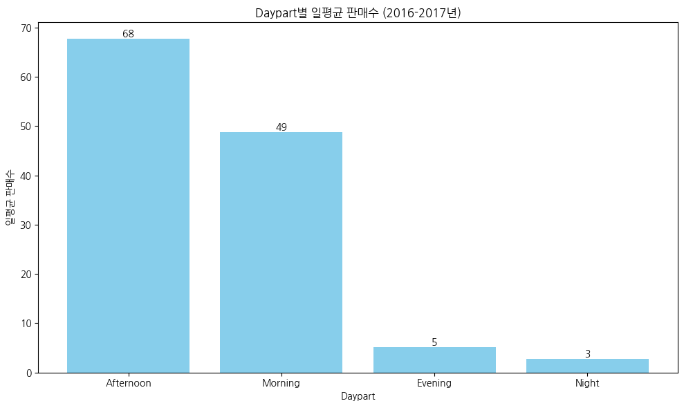
- 하루 중 대부분의 판매는 오전과 오후에 거래가 됐고, 그 이후는 현저하게 판매량이 적었다
- 매장 운영일수 대비 저녁장사는 소득이 적었다
1
2
3
4
5
6
7
8
9
10
11
12
13
14
15
16
17
18
19
20
21
22
23
24
25
26
27
28
29
30
# 월별 상위 10개 아이템 판매수 확인

# 월별 아이템 판매 수 집계
monthly_sales = df.groupby(['Month', 'Items']).size().reset_index(name='Quantity')

# 월별 상위 10개 아이템 추출
top_items = monthly_sales.groupby('Month').apply(lambda x: x.nlargest(10, 'Quantity')).reset_index(drop=True)

# 시각화
plt.figure(figsize=(20, 6))
colors = sns.color_palette('Paired')

# 각 월별로 상위 10개 아이템 시각화
for i in range(1, 13):  # 1부터 12까지 반복
    plt.subplot(2, 6, i)
    pr = top_items[top_items['Month'] == i]

    ax = sns.barplot(data=pr, x='Quantity', y='Items', palette=colors)

    for container in ax.containers:
        ax.bar_label(container)

    plt.xlabel('')
    plt.ylabel('')
    plt.title(f'{i}월 상위 10개 아이템 판매수', size=15)
    ax.spines[['top','right']].set_visible(False)

# 그래프 레이아웃 조정
plt.tight_layout()
plt.show()
1
2
/usr/local/lib/python3.10/dist-packages/ipykernel/ipkernel.py:283: DeprecationWarning: `should_run_async` will not call `transform_cell` automatically in the future. Please pass the result to `transformed_cell` argument and any exception that happen during thetransform in `preprocessing_exc_tuple` in IPython 7.17 and above.
  and should_run_async(code)
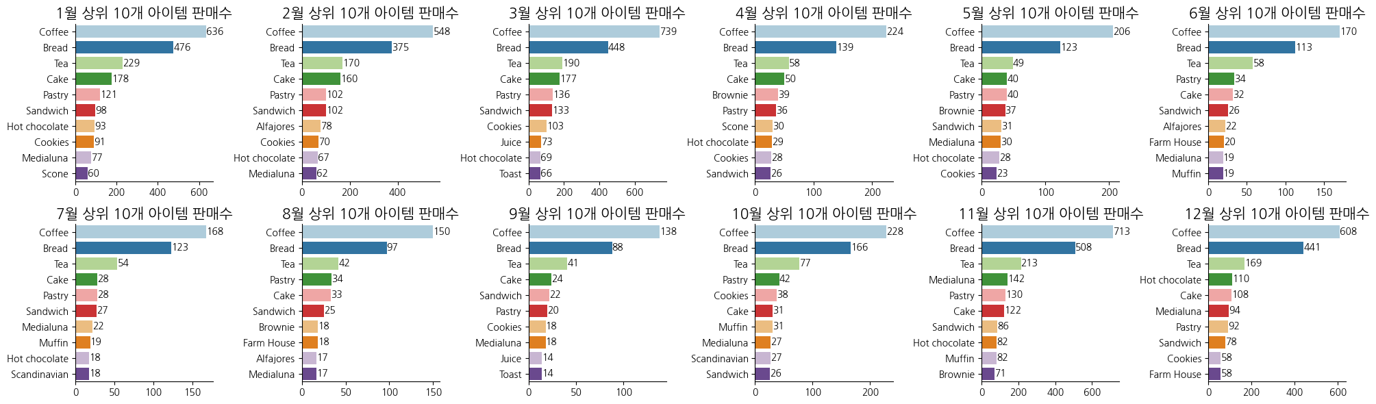
- 커피, 빵(bread), 차는 월별 고정 Top 3로 관찰됨
- 케이크, 페이스트리, 샌드위치, 브라우니가 Top 4~6에서 주로 관찰됨
- 메디아루나와 핫초코가 겨울에 어느정도 매출성과를 내고있음
1
2
3
4
5
6
7
8
9
10
11
12
13
14
15
16
17
18
19
20
21
22
23
24
25
26
27
28
29
30
31
32
33
34
35
# 요일별 일평균 판매수

# 요일별 운영일수 집계
operating_days = df.groupby('DayOfWeek')['Day'].nunique().reset_index(name='Operating Days')

# 요일별 판매수 집계
sales_per_day = df.groupby('DayOfWeek')['Items'].count().reset_index(name='Total Sales')

# 데이터 병합
weekly_data = operating_days.merge(sales_per_day, on='DayOfWeek')

# 요일별 일평균 판매수 계산 및 반올림
weekly_data['Average Sales'] = (weekly_data['Total Sales'] / weekly_data['Operating Days']).round().astype(int)

# 요일 순서 설정
day_order = ['Monday', 'Tuesday', 'Wednesday', 'Thursday', 'Friday', 'Saturday', 'Sunday']
weekly_data['DayOfWeek'] = pd.Categorical(weekly_data['DayOfWeek'], categories=day_order, ordered=True)

# 시각화
plt.figure(figsize=(12, 6))
ax = sns.barplot(data=weekly_data, x='DayOfWeek', y='Average Sales', color='skyblue')

# 그래프 위에 숫자 표시
for container in ax.containers:
    ax.bar_label(container)

# 그래프 설정
plt.xlabel('')
plt.ylabel('')
plt.title('요일별 일평균 판매수', size=15)

# 그래프 레이아웃 조정
plt.xticks(rotation=0)
plt.tight_layout()
plt.show()
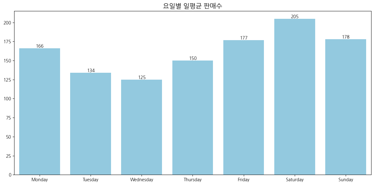
- 전반적으로 고르게 판매되고 있으며, 주말이 조금더 많은 판매를 하고있는것으로 관찰됨
연관분석 (Apriori 알고리즘)
1
2
# 최소지지도
df.info()
1
2
3
4
5
6
7
8
9
10
11
12
13
14
15
16
<class 'pandas.core.frame.DataFrame'>
RangeIndex: 18887 entries, 0 to 18886
Data columns (total 9 columns):
 #   Column         Non-Null Count  Dtype
---  ------         --------------  -----
 0   TransactionNo  18887 non-null  int64
 1   Items          18887 non-null  object
 2   Daypart        18887 non-null  object
 3   DayType        18887 non-null  object
 4   Year           18887 non-null  int32
 5   Month          18887 non-null  int32
 6   Day            18887 non-null  int32
 7   DayOfWeek      18887 non-null  object
 8   Hour           18887 non-null  int32
dtypes: int32(4), int64(1), object(4)
memory usage: 1.0+ MB
1
2
3
4
5
6
7
8
9
10
11
12
13
14
15
16
17
18
19
20
21
from mlxtend.frequent_patterns import apriori, association_rules

# 거래번호에 따라 아이템을 묶기
basket = df.groupby(['TransactionNo', 'Items'])['Items'].count().unstack().reset_index().fillna(0).set_index('TransactionNo')
basket = basket.applymap(lambda x: 1 if x > 0 else 0)  # 1은 아이템이 존재함을 나타내고, 0은 존재하지 않음을 나타냄

# Apriori 알고리즘 수행 (최소 지지도 : 0.025, 최소 향상도 1)
frequent_itemsets = apriori(basket, min_support=0.025, use_colnames=True)
rules = association_rules(frequent_itemsets, metric="lift", min_threshold=1)

# 결과를 Lift 기준으로 정렬
rules = rules.sort_values(by='lift', ascending=False)

# 소수점 둘째 자리까지 포맷팅
rules['support'] = rules['support'].round(2)
rules['confidence'] = rules['confidence'].round(2)
rules['lift'] = rules['lift'].round(2)

# 결과 출력
print("Frequent Itemsets:")
frequent_itemsets
1
2
3
4
5
6
7
8
9
/usr/local/lib/python3.10/dist-packages/ipykernel/ipkernel.py:283: DeprecationWarning: `should_run_async` will not call `transform_cell` automatically in the future. Please pass the result to `transformed_cell` argument and any exception that happen during thetransform in `preprocessing_exc_tuple` in IPython 7.17 and above.
  and should_run_async(code)


Frequent Itemsets:


/usr/local/lib/python3.10/dist-packages/mlxtend/frequent_patterns/fpcommon.py:109: DeprecationWarning: DataFrames with non-bool types result in worse computationalperformance and their support might be discontinued in the future.Please use a DataFrame with bool type
  warnings.warn(
| support | itemsets | |
|---|---|---|
| 0 | 0.036344 | (Alfajores) |
| 1 | 0.327205 | (Bread) |
| 2 | 0.040042 | (Brownie) |
| 3 | 0.103856 | (Cake) |
| 4 | 0.478394 | (Coffee) |
| 5 | 0.054411 | (Cookies) |
| 6 | 0.039197 | (Farm House) |
| 7 | 0.058320 | (Hot chocolate) |
| 8 | 0.038563 | (Juice) |
| 9 | 0.061807 | (Medialuna) |
| 10 | 0.038457 | (Muffin) |
| 11 | 0.086107 | (Pastry) |
| 12 | 0.071844 | (Sandwich) |
| 13 | 0.029054 | (Scandinavian) |
| 14 | 0.034548 | (Scone) |
| 15 | 0.034443 | (Soup) |
| 16 | 0.142631 | (Tea) |
| 17 | 0.033597 | (Toast) |
| 18 | 0.090016 | (Coffee, Bread) |
| 19 | 0.029160 | (Bread, Pastry) |
| 20 | 0.028104 | (Tea, Bread) |
| 21 | 0.054728 | (Cake, Coffee) |
| 22 | 0.028209 | (Coffee, Cookies) |
| 23 | 0.029583 | (Hot chocolate, Coffee) |
| 24 | 0.035182 | (Coffee, Medialuna) |
| 25 | 0.047544 | (Coffee, Pastry) |
| 26 | 0.038246 | (Coffee, Sandwich) |
| 27 | 0.049868 | (Coffee, Tea) |
1
2
print("\nAssociation Rules:")
rules
1
2
3
4
5
Association Rules:


/usr/local/lib/python3.10/dist-packages/ipykernel/ipkernel.py:283: DeprecationWarning: `should_run_async` will not call `transform_cell` automatically in the future. Please pass the result to `transformed_cell` argument and any exception that happen during thetransform in `preprocessing_exc_tuple` in IPython 7.17 and above.
  and should_run_async(code)
| antecedents | consequents | antecedent support | consequent support | support | confidence | lift | leverage | conviction | zhangs_metric | |
|---|---|---|---|---|---|---|---|---|---|---|
| 8 | (Coffee) | (Medialuna) | 0.478394 | 0.061807 | 0.04 | 0.07 | 1.19 | 0.005614 | 1.012667 | 0.305936 |
| 9 | (Medialuna) | (Coffee) | 0.061807 | 0.478394 | 0.04 | 0.57 | 1.19 | 0.005614 | 1.210871 | 0.170091 |
| 10 | (Coffee) | (Pastry) | 0.478394 | 0.086107 | 0.05 | 0.10 | 1.15 | 0.006351 | 1.014740 | 0.256084 |
| 11 | (Pastry) | (Coffee) | 0.086107 | 0.478394 | 0.05 | 0.55 | 1.15 | 0.006351 | 1.164682 | 0.146161 |
| 12 | (Coffee) | (Sandwich) | 0.478394 | 0.071844 | 0.04 | 0.08 | 1.11 | 0.003877 | 1.008807 | 0.194321 |
| 13 | (Sandwich) | (Coffee) | 0.071844 | 0.478394 | 0.04 | 0.53 | 1.11 | 0.003877 | 1.115384 | 0.109205 |
| 2 | (Cake) | (Coffee) | 0.103856 | 0.478394 | 0.05 | 0.53 | 1.10 | 0.005044 | 1.102664 | 0.102840 |
| 3 | (Coffee) | (Cake) | 0.478394 | 0.103856 | 0.05 | 0.11 | 1.10 | 0.005044 | 1.011905 | 0.176684 |
| 4 | (Coffee) | (Cookies) | 0.478394 | 0.054411 | 0.03 | 0.06 | 1.08 | 0.002179 | 1.004841 | 0.148110 |
| 5 | (Cookies) | (Coffee) | 0.054411 | 0.478394 | 0.03 | 0.52 | 1.08 | 0.002179 | 1.083174 | 0.081700 |
| 6 | (Hot chocolate) | (Coffee) | 0.058320 | 0.478394 | 0.03 | 0.51 | 1.06 | 0.001683 | 1.058553 | 0.060403 |
| 7 | (Coffee) | (Hot chocolate) | 0.478394 | 0.058320 | 0.03 | 0.06 | 1.06 | 0.001683 | 1.003749 | 0.109048 |
| 0 | (Bread) | (Pastry) | 0.327205 | 0.086107 | 0.03 | 0.09 | 1.03 | 0.000985 | 1.003306 | 0.050231 |
| 1 | (Pastry) | (Bread) | 0.086107 | 0.327205 | 0.03 | 0.34 | 1.03 | 0.000985 | 1.017305 | 0.036980 |
1
2
3
4
5
selected_rules = rules[['antecedents', 'consequents', 'support', 'confidence', 'lift']]
selected_rules['support'] = selected_rules['support'].round(2)
selected_rules['confidence'] = selected_rules['confidence'].round(2)
selected_rules['lift'] = selected_rules['lift'].round(2)
selected_rules.sort_values(by='lift', ascending=False)
1
2
/usr/local/lib/python3.10/dist-packages/ipykernel/ipkernel.py:283: DeprecationWarning: `should_run_async` will not call `transform_cell` automatically in the future. Please pass the result to `transformed_cell` argument and any exception that happen during thetransform in `preprocessing_exc_tuple` in IPython 7.17 and above.
  and should_run_async(code)
| antecedents | consequents | support | confidence | lift | |
|---|---|---|---|---|---|
| 8 | (Coffee) | (Medialuna) | 0.04 | 0.07 | 1.19 |
| 9 | (Medialuna) | (Coffee) | 0.04 | 0.57 | 1.19 |
| 10 | (Coffee) | (Pastry) | 0.05 | 0.10 | 1.15 |
| 11 | (Pastry) | (Coffee) | 0.05 | 0.55 | 1.15 |
| 12 | (Coffee) | (Sandwich) | 0.04 | 0.08 | 1.11 |
| 13 | (Sandwich) | (Coffee) | 0.04 | 0.53 | 1.11 |
| 2 | (Cake) | (Coffee) | 0.05 | 0.53 | 1.10 |
| 3 | (Coffee) | (Cake) | 0.05 | 0.11 | 1.10 |
| 4 | (Coffee) | (Cookies) | 0.03 | 0.06 | 1.08 |
| 5 | (Cookies) | (Coffee) | 0.03 | 0.52 | 1.08 |
| 6 | (Hot chocolate) | (Coffee) | 0.03 | 0.51 | 1.06 |
| 7 | (Coffee) | (Hot chocolate) | 0.03 | 0.06 | 1.06 |
| 0 | (Bread) | (Pastry) | 0.03 | 0.09 | 1.03 |
| 1 | (Pastry) | (Bread) | 0.03 | 0.34 | 1.03 |
- 빵이나 디저트를 구매하는 고객 2명 중 1명은 커피를 함께 구매한다
- 커피와 자주 구매되는 품목들(메디아루나, 페이스트리, 케이크 등)을 세트로 판매하는 방안을 검토해본다
1
2
3
4
5
6
7
8
9
10
11
12
13
14
15
16
17
18
19
20
21
22
23
24
25
26
27
28
29
30
31
32
33
34
35
36
37
38
39
40
41
42
43
44
45
46
# 네트워크그래프 시각화
import networkx as nx
from mlxtend.frequent_patterns import apriori, association_rules

# 거래번호에 따라 아이템을 묶기
basket = df.groupby(['TransactionNo', 'Items'])['Items'].count().unstack().reset_index().fillna(0).set_index('TransactionNo')
basket = basket.applymap(lambda x: 1 if x > 0 else 0)

# Apriori 알고리즘 수행 (최소 지지도 : 0.025, 최소 향상도 1)
frequent_itemsets = apriori(basket, min_support=0.025, use_colnames=True)
rules = association_rules(frequent_itemsets, metric="lift", min_threshold=1)

# 네트워크 그래프 생성
G = nx.DiGraph()

# 노드와 엣지 추가
for _, rule in rules.iterrows():
    G.add_node(rule['antecedents'], label=', '.join(rule['antecedents']))
    G.add_node(rule['consequents'], label=', '.join(rule['consequents']))
    G.add_edge(rule['antecedents'], rule['consequents'], weight=rule['lift'], lift=rule['lift'])

# 노드 레이블 설정
labels = {node: G.nodes[node]['label'] for node in G.nodes()}

# 그래프 시각화
plt.figure(figsize=(12, 8))
pos = nx.spring_layout(G)  # 위치 설정
edges = G.edges(data=True)

# 엣지 그리기
nx.draw_networkx_edges(G, pos, edgelist=edges, width=[edge[2]['weight'] for edge in edges], alpha=0.5)

# 노드 그리기 (연한 갈색으로 설정)
nx.draw_networkx_nodes(G, pos, node_size=2000, node_color='salmon')

# 노드 레이블 그리기
nx.draw_networkx_labels(G, pos, labels, font_size=10)

# 엣지 위에 Lift 값 표시
edge_labels = {(rule['antecedents'], rule['consequents']): f"{rule['lift']:.2f}" for _, rule in rules.iterrows()}
nx.draw_networkx_edge_labels(G, pos, edge_labels=edge_labels, font_color='black')

# 그래프 제목
plt.title('네트워크그래프', size=15)
plt.axis('off')  # 축 숨기기
plt.show()
1
2
3
4
/usr/local/lib/python3.10/dist-packages/ipykernel/ipkernel.py:283: DeprecationWarning: `should_run_async` will not call `transform_cell` automatically in the future. Please pass the result to `transformed_cell` argument and any exception that happen during thetransform in `preprocessing_exc_tuple` in IPython 7.17 and above.
  and should_run_async(code)
/usr/local/lib/python3.10/dist-packages/mlxtend/frequent_patterns/fpcommon.py:109: DeprecationWarning: DataFrames with non-bool types result in worse computationalperformance and their support might be discontinued in the future.Please use a DataFrame with bool type
  warnings.warn(
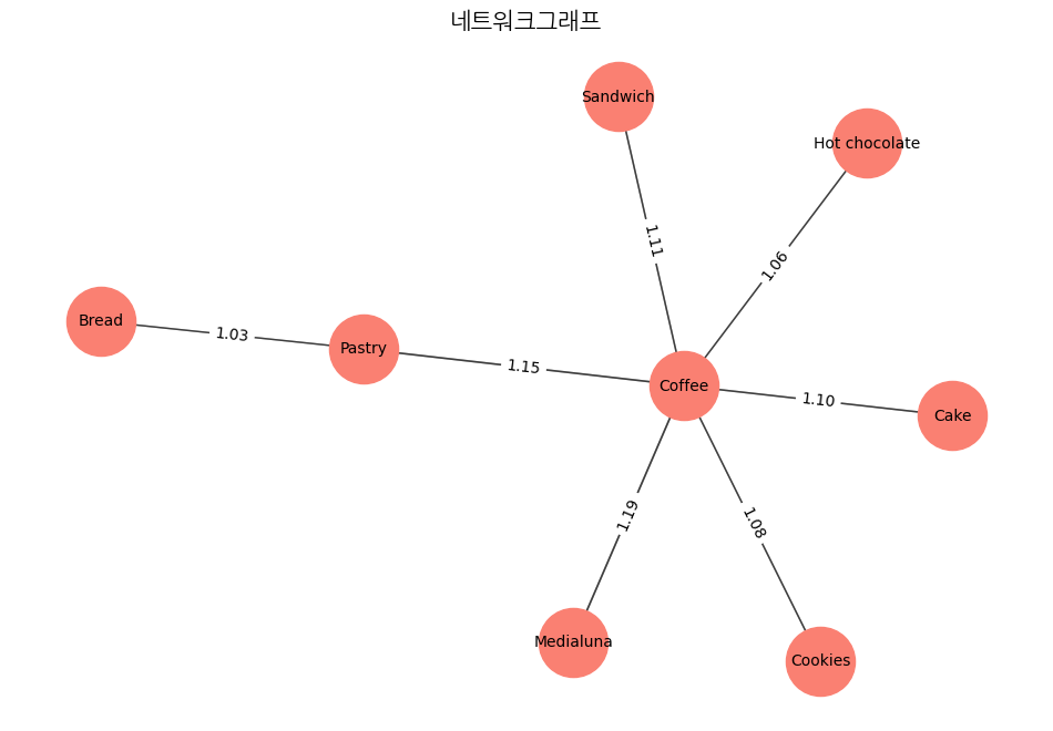
- 커피는 다른 아이템들과 연관성이 뚜렷하게 높은것으로 관찰됨. 다른아이템들과 함께 자주 구매되고 있음
- 커피를 구매하는 고객이 빵(bread) 또는 페이스트리를 구매하는 경향이 관찰됨
This post is licensed under CC BY 4.0 by the author.